Determining a composite value for the saturated hydraulic conductivity in a recharge area of the Guarani Aquifer System, using pedotransfer functions

Determinação de um valor composto para a condutividade hidráulica saturada em uma área de recarga do Sistema Aquífero Guarani, utilizando funções pedotransfer

ABSTRACT

The saturated hydraulic conductivity (K_s) is an essential property for modeling water and contaminants movement into aquifers. However, K_s is extremely variable, even when considering nearby locations, which poses a challenge for modeling at catchment scales. Field measurements of K_s are most of the time expensive, time-consuming and labor-intensive. This study aimed to obtain, for modeling purposes, and using pedotransfer functions (PTFs), a composite value of K_s at a catchment scale, in a recharge area of the Guarani Aquifer System. Soil samples were taken across the study area, and the K_s for each sampling point were determined by several PTF methods. At the same locations, K_s field measurements were taken using a Guelph permeameter. Average values of K_s for all the sampling points calculated by PTFs were similar to the average value obtained by field measurements. The use of PTFs proved to be a faster and simpler method to efficiently determine the K_s value for the watershed and to capture the stochastic variation in terms of soil pore combination at the watershed scale.

Keywords:
Guarani Aquifer System; Hydraulic conductivity; Pedotransfer function; Recharge area

RESUMO

A condutividade hidráulica saturada (K_s) é uma propriedade essencial para modelagem do fluxo de água e contaminantes da zona não saturada em direção aos aquíferos. Entretanto, K_s é extremamente variável, mesmo considerando-se locais muito próximos, o que torna a modelagem em escala de bacia de drenagem um desafio. Medições de K_s em campo são na maioria das vezes dispendiosas, demoradas e trabalhosas. O objetivo desse estudo é obter, para fins de modelagem computacional, e por meio de funções de pedotransferência (FPTs), um valor representativo de K_s para uma área de recarga do Sistema Aquífero Guarani. Amostras de solo foram coletadas por toda área de estudo e os valores de K_s em cada ponto de amostragem determinados por meio de FPTs. Nos mesmos pontos, foram feitas medições de K_s por meio de um permeâmetro Guelph. Os valores médios de K_s calculados por meio de FPTs para todos os pontos de amostragem foram semelhantes aos valores médios obtidos pelas medições de campo. O uso de FPTs provou ser um método mais rápido e simples para determinar com eficiência o valor de K_s da área de recarga e para capturar a variação estocástica em termos de combinação de poros do solo na escala considerada.

Palavras-chave:
Sistema Aquífero Guarani; Condutividade hidráulica; Funções de pedotransferência; Área de recarga

INTRODUCTION

The unsaturated zone is the link between precipitation and groundwater, therefore knowledge of near-surface hydraulic properties in recharge areas is essential to understand the movement of water and contaminants into the aquifer. Determining soil hydraulic properties is a prerequisite to physically model transient water flow and solute transport in the unsaturated zone (Sprenger et al., 2015).

Although water movement at the subsurface occurs mostly at unsaturated conditions, the saturated hydraulic conductivity (K_s) is considered a fundamental soil property for water and solute transport in the unsaturated zone (De Pue et al., 2019; Mesquita & Moraes, 2004; Vienken & Dietrich, 2011). K_s not only governs the flow rate of water under a hydraulic gradient as specified by the Darcy equation for saturated conditions, but also acts as a scaling factor in many unsaturated flow and transport applications that involve pore-size distribution models (Zhang & Schaap, 2019).

However, hydraulic conductivity is known to be one of the most variable of all geotechnical properties (Mbonimpa et al., 2002). Within the same soil class or geological unit, K_s values in nearby sites can vary by several orders of magnitude (Mesquita & Moraes, 2004).

There are several available methods for the determination of _Ks, either in a laboratory or through field investigation. Common field methods for estimation of K_s make use of ring infiltrometers and borehole permeameters. Ring infiltrometers can be used to pond water on the soil surface and measure the infiltration rate. Borehole permeameters consist of a Mariotte siphon that maintains water at a constant level in a borehole and allows measurement of the steady flow rate into the soils (Radcliffe & Simunek, 2010). Laboratory methods implicate in collecting soil samples using stainless steel rings. The K_s can be measured in the laboratory by using a constant head or a falling head method. For the constant head method, a constant hydraulic head difference is maintained across the soil sample for the entire duration of measurement, whereas in a falling head method the hydraulic head varies over time (Lal & Shukla, 2004). Most methods are time-consuming and laborious, might require large volumes of water, and can be too expensive or impractical for large scales (Cornelis et al., 2001; De Pue et al., 2019; Odong, 2007; Vereecken et al., 2010).

Successful hydrological model predictions depend on appropriate framing of scale and the spatial-temporal accuracy of input parameters describing soil hydraulic properties (Libohova et al., 2018). Modeling water movement in the unsaturated zone presents the challenge of correctly depicting its hydraulic properties. Considering the high variability of such properties, it is impractical at watershed scales to measure them at every few square meters. Instead, a representative value for the entire area considerably reduces model complexity while also being less labor-intense.

Considering watershed scales, soil properties related to groundwater flow and transport vary according to parent material, vegetation, and land use; which in turn affect characteristics such as macroporosity, layering, and aggregation, and therefore, vertical water movement (Bosch & West, 2010; Kutílek & Nielsen, 1994). Trying to use point‐scale physics at the basin scale implies that both the media and the boundary conditions should be known spatially at the scale of the equations. This, in turn, requires prohibitive amounts of input data, which in most cases goes far beyond practical limitations even for small experimental plots (Zehe et al., 2006).

To evade these difficulties, and considering their importance in the fields of hydrogeology, petroleum geology, and wastewater engineering, there has been substantial work towards developing empirical relationships between soil hydraulic properties and various, more easily measurable, attributes of the porous medium (Sperry & Peirce, 1995). These so-called pedotransfer functions (PTFs) are surrogate analyses relating soil hydraulic functions to basic and simple soil data such as the content of clay, silt, sand, organic matter, and values of bulk density or porosity (Kutílek & Nielsen, 1994). PTFs are usually obtained using various mathematical and statistical approaches, such as regression or neural network analysis. PTFs can be used to predict either soil hydraulic properties directly, such as the water content at specified pressure heads and the saturated hydraulic conductivity, or parameters in the analytical models used for soil hydraulic properties (Radcliffe & Simunek, 2010).

The Guarani Aquifer System (GAS) is considered one of the most important hydrostratigraphic units of South America (Sindico et al., 2018), providing potable water to more than 90 million people (Gastmans et al., 2010). It is a typical example of a transboundary aquifer, located in the western region of South America, covering an area of about 1.1 million Km² (Organização dos Estados Americanos, 2009). It is essentially a confined or semiconfined aquifer. Only about 10% of the GAS is represented by outcrop area, with sedimentary rock strata of sandstone and a basaltic confinement layer (Rabelo & Wendland, 2009). GAS outcrop formations in the central portion of São Paulo occur in a continuous North-South strip, corresponding to one of the most important recharge areas for the aquifer.

Previous studies carried out regarding GAS hydraulic conductivity usually emphasized only the saturated portion of the GAS, and/or its geological formations (Soares et al., 2008; Rabelo & Wendland, 2009). This paper is concerned with a somehow neglected yet important GAS characteristic, which is the movement of water and contaminants through the unsaturated zone of the aquifer.

The main purpose of this study is to use PTF functions based on grain-size analysis, to obtain a composite value of K_s for a catchment at a recharge area of the Guarani Aquifer System. For that matter, samples were collected throughout the catchment across different geological formations and soil types. The assessment of the PTF results was performed comparing their results with direct field measurements performed with a Guelph permeameter (Reynolds & Elrick, 1986).

Some research questions have guided this study: a) Are PTFs a good surrogate for K_s field measurements, and how do they vary considering the number of samples? b) Which PTFs are more accurate in determining K_s values considering field measurements? c) How does the spatial resolution influence the results? d) What are the main limitations of the use of PTFs?

MATERIAL AND METHODS

Study area

The Jacaré-Pepira basin is located in the central region of the state, draining an area of approximately 2500 km² in the portion upper Tietê-Jacaré basin (Tundisi et al., 2008).

The area of interest is a sub-basin of the Jacaré-Pepira basin, situated in its upper portion and most of its outcropping geological units correspond to Mesozoic sediments from Botucatu and Piramboia formations. It also presents basaltic outcrops from the Serra Geral formation, and tertiary sediments at its higher portions (Batista et al., 2018). The geological and pedological characteristics and location of the sampling points are illustrated in Figure 1.

Figure 1
Location of the GAS in South America, GAS outcrops, and study area in the State of São Paulo. Below - Maps of the study area: Digital Elevation Model (left), Soil Types (Center), Geological Units (right).

The Piramboia Formation consists of silty-clayish sandstones of aeolian and fluvial origins, and the Botucatu Formation consists of well-sorted sandstones of aeolian origin (Sracek & Hirata, 2002). The Serra Geral formation corresponds to successive layers of basaltic volcanic activity spills from the Cretaceous period (Rabelo & Wendland, 2009). The soils in the area correspond in more than 90% to Oxisols (Hapludox and Haplustox) and Entisols (Quartzipsamments). Other soil occurrences include Ultisols, Entisols (Aquents), and Alfisols. Oxisols are highly weathered soils with oxic subsurface horizon, very high in clay-sized particles, dominated by hydrous oxides of iron and aluminum. Entisols are weekly developed mineral soils without natural subsurface horizons. Ultisols are characterized by a B horizon with loamy-sand texture, with less than 35% of the exchange capacity, where there has been an increment of the clay fraction. Alfisols are characterized by a subsurface diagnostic horizon in which silicate clay was accumulated by illuviation and its cation exchange capacity is above 35% (Brady & Weil, 2014).

Sampling

Sampling points were chosen in order to have a spatial distribution with coverage throughout the study area, considering its geological formations and the ease of access to the locations. Based on these criteria a total of 34 sampling locations were chosen as indicated in Figure 1. To evaluate the results of PTFs, field measurements of K_s were determined at the same sampling locations using the Guelph permeameter.

Grain size distribution curve

Porosity, hydraulic conductivity, and permeability are hydrogeological parameters that greatly depend on the size of sediment grains and the percentage of various sediment fractions (Kresic, 2007). The most used method to determine grain size distribution consists of separating the fractions of the sediments through a set of sieves with different diameters. Sample grain size distribution was determined by combining the sieve and sedimentation analysis methods, which consists in measuring the weight of each particle size interval, expressing it as a percentage of the sample’s total weight. In this case, the set of sieves were size #4, #10, #16, #30, #40, #50, #60, #100, #200 and #230, which have diameters varying from 4.76 to 0.063 millimeters (mm). The determination of grain size distribution for silt and clay (grains smaller than 0.075 mm), was performed when the percentage of fines was above 15%. The finer particles were stirred and left for a 48 hours decantation in a vertical cylinder of water. During the decantation, density measurements were taken with a hydrometer, under monitored conditions, at each defined time interval. The diameter of the grains was determined from the suspension density, which progressively decreases over time at a given elevation (Kresic, 2007). The grain size distribution curve is then plotted in a semilogarithmic graph, with the cumulative percent coarser by weight plotted on the vertical scale and the diameter of grains on a horizontal logarithmic scale.

Guelph permeameter

The use of the Guelph permeameter to determine hydraulic conductivity is well documented in the literature (Appels et al., 2015; Guzman et al., 2019; Oliva et al., 2005; Soto & Kiang, 2018). This method provides simultaneous in situ measurements of field-saturated hydraulic conductivity, and matric flux potential. It measures the steady-state rate of water flow out of a shallow, cylindrical well in which a constant depth of water (pressure head) is maintained. A Mariotte bottle device is used to maintain the depth of water and to measure the rate of water flow (Kanwar et al., 1989). More specific details about the method can be found in Reynolds & Elrick, (1986) and Ghosh & Pekkat (2019).

Empirical relationship between grain-size and hydraulic conductivity

The movement of water through the media depends on the hydraulic gradient; size, geometry, and distribution of pores between solid grains (Mbonimpa et al., 2002). Therefore, quite a few empirical formulas for calculating hydraulic conductivity using grain size analysis are available in the literature (Fetter, 2014; Song et al., 2009; Vienken & Dietrich, 2011; Zhang & Schaap, 2019).

The applicability of each method depends on the characteristics of the soil or sediment. For instance, some methods present better results with soils or sediments composed of sand particles, while others are more efficient for soil or sediments uniformly graded regardless of the predominant texture fraction. In this study, we took the liberty to use several PTF methods even considering that not all methods apply to all samples.

Most empirical equations currently in use are expressed based on the following general equation (Song et al., 2009):

$K_s=\frac{g}{v}.C.f\left(n\right).d_e{}^2$ (1)

where K_s is the saturated hydraulic conductivity, g is the acceleration due to gravity, v is the kinematic viscosity of the fluid (water), C is a dimensionless coefficient that depends on various parameters of the porous medium, such as grain shape, structure, and heterogeneity, f(n) is a function of porosity n, and d_e is the effective grain size. In this study, K_s was calculated in cm/s, g in cm/s², v in cm²/s, and d_e in cm.

Porosity (n) may be derived from the empirical relationship with the coefficient of grain uniformity (U) as follows (Vienken and Dietrich, 2011):

$n=0.255\cdot \left(1+{0.83}^U\right)$ (2)

where U is the uniformity coefficient is given by:

$U=\frac{d_{60}}{d_{10}}$ (3)

where, d₆₀ and d₁₀ are the particle diameters derived from cumulative distribution and represent size fractions at which 60% and 10%, respectively, of the sample by weight is composed of grains of smaller size (Ayers et al., 1998).

In this study, seven empirical methods were selected, Table 1 summarizes these formulas and their applicability.

Table 1
Formulas and applicability of the empirical grain-size methods.

Method	Formula	f(n)	Effective grain diameter (de)	Value of C	Domain of applicability
Shepherd(1)	$K=C{d}_{50}{}^{1.5}$	1	d50	100	0.01mm< de <10mm
Hazen Complete(2)	$K=\frac{g}{v}\left(6\times {10}^{-4}\right)\left[1+10\left(n-0.26\right)\right]d_{10}{}^2$	1+10(n-0.26)	d10	6x10-4	0.1mm<de<3mm
Hazen(1)	$K=100d_{10}{}^2$	1	d10	100	0.1mm<de<3mm
Kozeny-Carman(3)	$K=\frac{g}{v}\left(8.3\times {10}^{-3}\right)\left(\frac{n^3}{1-n^2}\right)d_{10}{}^2$	$\frac{n^3}{1-n^2}$	d10	8.3x10-3	large grain sands
Beyer(3)	$K=\frac{g}{v}6x{10}^{-4}\left(log\frac{500}{U}\right)d_{10}{}^2$	1	d10	$6x{10}^{-4}\left(log\frac{500}{U}\right)$	0.06mm<de<0.6mm
Slichter(3)	$K=\frac{g}{v}\left(1\times {10}^{-2}\right)n^{3.287}{d}_{10}{}^2$	$n^{3.287}$	d10	1x10-2	0.01mm<de<0.5mm
Terzaghi(3)	$K=\frac{g}{v}\left(10.7\times {10}^{-3}\right){\left(\frac{n-0.13}{\sqrt[3]{1-n}}\right)}^2{d}_{10}{}^2$	${\left(\frac{n-0.13}{\sqrt[3]{1-n}}\right)}^2$	d10	6.1x10-3 <C<10.7x10-3	large grain sands
USBR(3)	$K=\frac{g}{v}\left(7.34\times {10}^{-4}\right)d_{20}{}^{2.3}$	1	d20	7.34x10-4	U<5

• Obs: ⁽¹⁾Fetter (2014);
• ⁽²⁾Vienken & Dietrich (2011);
• ⁽³⁾Song et al. (2009).

Based on the grain size distribution curves, the effective grain diameters d₅₀, d₂₀, and d₁₀ represent size fractions at which 50%, 20%, and 10%, respectively, of the sample, is composed of grains of smaller size. For all methods, the value of gravitational acceleration near the earth’s surface (g) is assumed to be 9.806 m/s² and the water temperature being 20 °C, which corresponds to the dynamic viscosity (v) value of 1.004x10^-6 m/s², respectively.

The Willmott index

To evaluate the efficiency of the results obtained by the PTFs, the results for each sampling point were compared with the values of K_s obtained by the Guelph permeameter, using the Willmott index of agreement (Willmott, 1981) according to the following equation:

$d=1-\left[\frac{{{\displaystyle \sum }}_{i=1}^n{(P_i-O_i)}^2}{{{\displaystyle \sum }}_{i=1}^n{\left(\left|P_i-O_m\right|+\left|O_i-O_m\right|\right)}^2}\right]$ (4)

where: d – Willmott index; P_i – Calculated values; O_i – Observed values; O_m – average of observed values; n – the total number of values

Values of d close to zero indicate no agreement of the model results with field results and values close to one imply total agreement.

Statistical evaluation

The Kruskal-Wallis (KW) test was used to identify similarities among the PTFs. The KW test is similar to the parametric analysis of variance but is performed on data ranks rather than data values, and it is not restricted by the assumption of normality. A significant KW test result (a p-value smaller than 0,05), indicates that the sample population distribution of at least one sample differs from another (Krueger et al., 2015). The Shapiro-Wilk test of normality was applied to check for the possible normality distribution of field and PTFs results.

RESULTS AND DISCUSSIONS

Soil texture and granulometry

Grain size analysis shows that for most of the sampling points, coarse grains predominate over finer fractions. Sands, loamy sands, and sandy loams are the predominant soil texture in the area, except for a minor portion that corresponds to the Serra Geral Formation with clayey soils (Figure 2).

Figure 2
Soil texture triangle and texture classification of sampling the points (red), based on grain-size analysis. Source: Soil Texture Calculator (U.S. Department of Agriculture, 2020).

It is possible to observe, that the granulometry of the samples are relatively homogenous despite covering different geological formations. Only the samples collected on the Serra Geral formation show high clay content, and a few samples located on the tertiary deposits present intermediate (about 20%) clay content.

Guelph permeameter results

The results of direct field measurement with the permeameter showed variations of several orders of magnitude, ranging from a minimum of 5.29x10^-6 cm/s to a maximum of 2.00x10^-2 cm/s, with an average of 2.97x10^-3 cm/s. Compared with other studies, Engelbrecht et al. (2020), through pumping tests calculated the average value of K_s for the GAS aquifer ranging from 2,23x10^-3 cm/s to 2,28x10^-3 cm/s. In the same study, using the Kozeny-Carman method, K_s estimates for the Botucatu and Piramboia formations were respectively of 3.37 cm/s and 2.71 cm/s. Rabelo & Wendland (2009), using numerical modeling to study GAS aquifer recharge at the sub-basins of Jacaré-Pepira and Jacaré Guaçu; calculated the average K_s value of these sub-basins as 2,78x10^-3 cm/s, varying from 2,00x10^-4 cm/s to 5,00x10^-3 cm/s. Sracek & Hirata (2002), report K_s values ranging from 2,0x10^-4 cm/s to 1,9x10^-1 cm/s for the Piramboia and Botucatu formations in the Guarani Aquifer. Zuquette & Palma (2006), using double-ring infiltration tests to measure hydraulic conductivity on the Botucatu and Serra Geral formations reported K_s values varying from 1.48x10^-6 to 3.65x10^-5 cm/s for the unconsolidated basalt of Serra Geral, and ranging from 3.2x10^-3 cm/s to 2.01x10^-5 cm/s for the sandy materials of Botucatu formation.

The sandstones of the Jurassic period of aeolian origin (Botucatu formation), have higher hydraulic conductivity and are the best reservoirs of the Jacaré system basins, while the Triassic sandstones of fluvio-lacustrine/aeolian origin (Piramboia Formation), usually have larger amounts of clay diminishes in relative terms their hydraulic efficiency (Rabelo & Wendland, 2009).

Interestingly in this study, the two lowest values of K_s were measured in loamy sands and sandy soils, whereas one would normally expect them to be found in clayey soils. Also, the variation of measured Ks values reached more than one order of magnitude even when considering sampling points within the same textural class, geological formation, or land use. A Shapiro-Wilk test of normality shows that the natural log of K_s has a p-value of 0.3133. The K_s results, separated by geological formation are presented in Table 2.

Table 2
Ks values by geological formation.

Formation	Ks medio (cm/s)	Ks maximum (cm/s)	Ks minimum (cm/s)
Piramboia	1.749x10-3	5.790x10-3	2.670x10-3
Botucatu	2.865x10-3	1.010x10-2	1.330x10-4
Serra Geral	7.844x10-4	1.820x10-3	5.291x10-6
Tertiary deposits	1.718x10-3	3.400x10-3	8.43x10-4

Slightly higher K_s values were measured for the Botucatu formation compared to Piramboia formation, and as expected lower K_s values for the clayey outcrops of Serra Geral. Measurements of K_s by Oliva et al. (2005), using a Guelph permeameter in the Rio Claro formation, which has similar characteristics as the tertiary deposits of the study area, provided K_s values ranging from 8.0x10^-4 cm/s to 4,9x10^-3 cm/s.

When the results are separated by slope, K_s values are higher for areas with smaller slopes as indicated in Table 3.

Table 3
Ks values by slope.

Slope	Ks average (cm/s)	Ks maximum (cm/s)	Ks Minimum (cm/s)
0-5	1.551x10-3	5.79x10-3	1.640x10-4
5-10	2.317x10-3	2.010x10-2	2.330x10-4
>10	5.898x10-4	1.680x10-3	5.290x10-6

PTF results

Grain size analysis provided the information to evaluate from the PTF methods chosen which ones are more suitable, considering their range of applicability and given granulometric characteristics. Based on grain size results, the Shepherd method is the most suitable for the area, since it applies to all samples, except for the two clayey from the Serra Geral formation. The Slitcher method also has applicability to most samples except for the tertiary deposits and the Serra Geral formation. However, as previously mentioned, we took the liberty to use several PTFs methods even if they are not perfectly suitable for all samples.

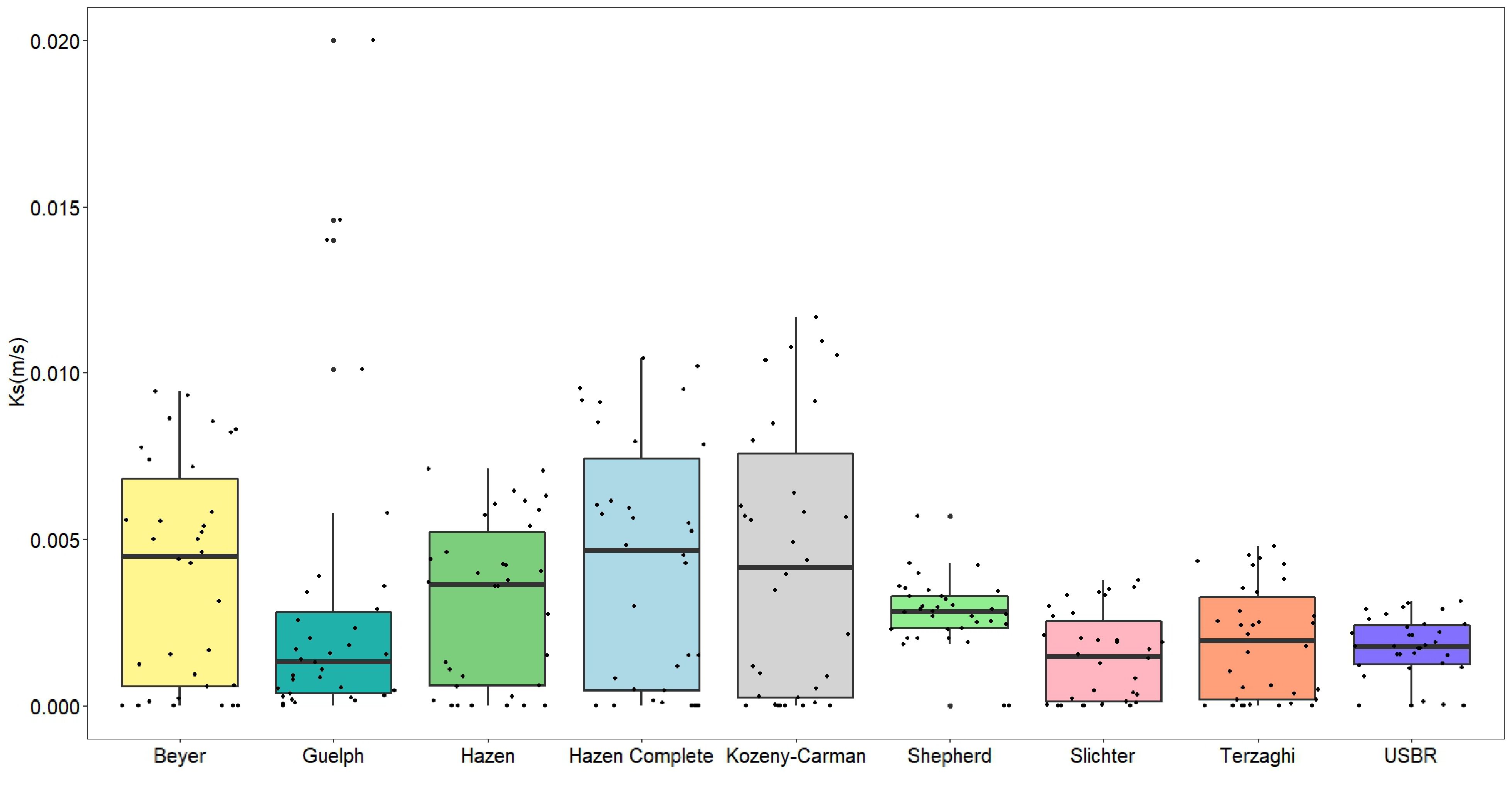
The K_s calculated from PTFs present large variations from one method to another. Values for the same sampling point varied up to two orders of magnitude depending on the PTF applied. A boxplot of K_s values obtained by PTFs and the Guelph permeameter is shown in Figure 3.

Figure 3
Boxplot of Ks results for different methods.

Applying the Shapiro-Wilk test of normality, none of the PTF results showed a normal distribution at a 0.05 α-level.

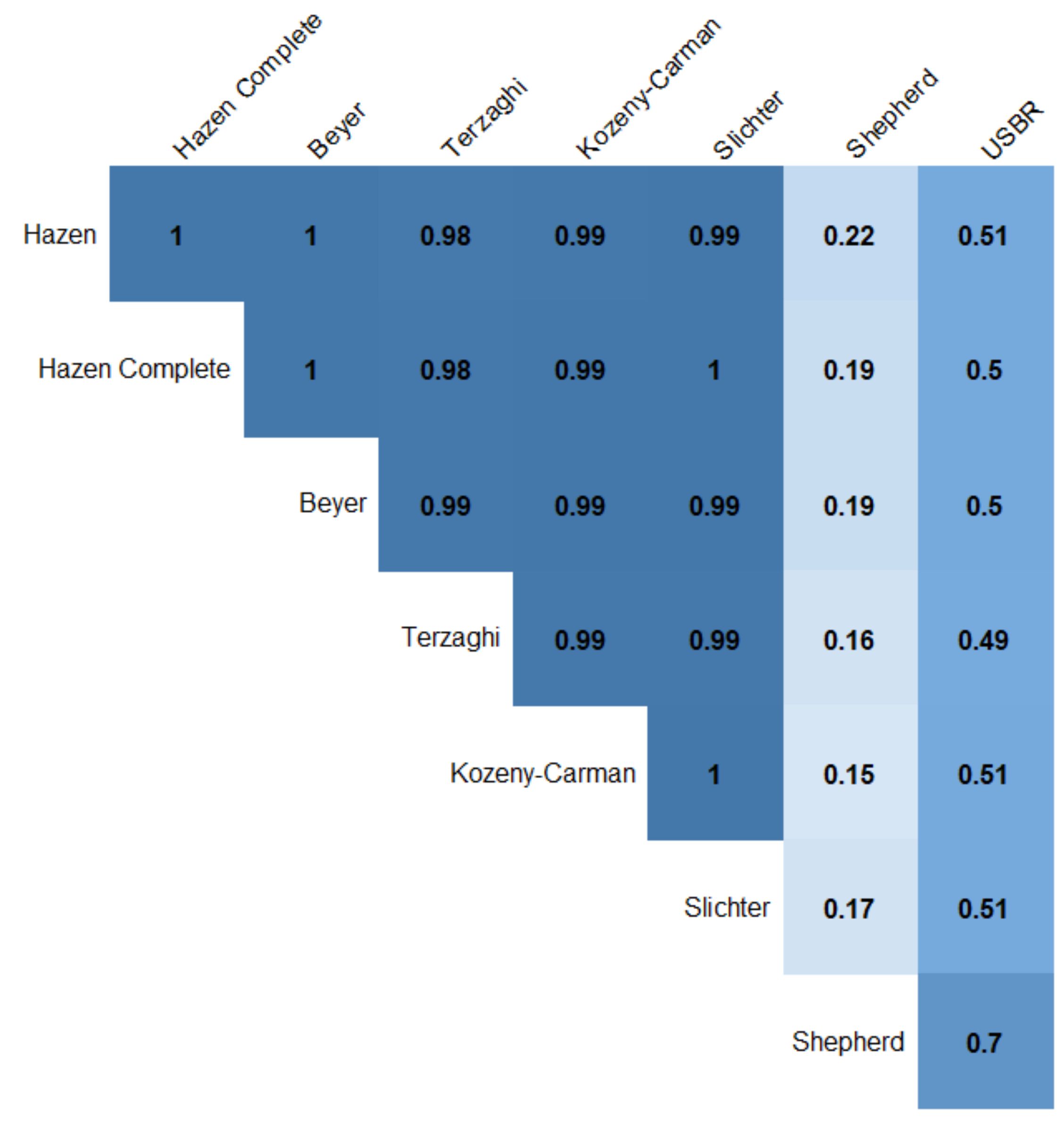
The correlation between measured K_s values on the field and the ones obtained by PTFs is weak for all methods considered. The best correlation coefficient between measured K_s values measured on the field and the ones obtained by PTFs is of 0.292 for the Hazen method. On the other hand, the correlation among the PTFs is strong in most cases, except for Shepherd and USBR methods (Figure 4), which do not consider the porosity factor in their formulas.

Figure 4
Correlation of Ks values among PTF methods.

Another peculiarity is that among the methods used, these are the only ones that do not use d₁₀ as the effective grain size; the USBR method uses d₂₀ and the Shepherd method uses d₅₀.

Willmott index results

Comparison of K_s values obtained by PTFs at each sampling point, with K_s values measured with the Guelph permeameter also shows little agreement. The difference in some cases reaches three or four orders of magnitude. Consequently, the Willmott agreement index in all cases is moderate at best (Table 4). About twelve of the sampling points consistently showed high differences of two or more orders of magnitude, between estimated and measured K_s values. These points do not have a common characteristic that could explain this pattern, such as texture, porosity, level of uniformity, or percentage of fines or topography. However, they all fall outside the range of applicability for most PTF methods, except for the Shepherd method.

Table 4
Willmott Index results.

PTF	d- Willmott index
Shepherd	0.473
Hazen	0.431
Hazen Complete	0.505
Kozeny- Carman	0.403
Beyer	0.435
Slichter	0.453
Terzaghi	0.449
USBR	0.527

The correlation of natural logarithms of K_s values calculated by PTFs presents slightly better results when compared with the natural logarithm of field measurements (Table 5).

Table 5
Correlation between field results and PTFs (α=0.05).

PTFs	Ln Guelph Permeameter
Ln Shepherd	0.122
Ln Hazen	0.410
Ln Hazen Complete	0.418
Ln Kozeny - Carman	0.420
Ln Beyer	0.419
Ln Slichter	0.419
Ln Terzaghi	0.426
Ln USBR	0.369

Kruskal-Wallis statistics

Given the wide range of values obtained either by field measurements or by PTFs, and the discrepancies of K_s values for the same sample location; the (KW) H test was used to exam the significance of such differences. Despite the limitations in applicability, all methods except the Hazen Complete presented a KW p-value above 0.05 when compared to field measurements., therefore there is no reason to conclude that other distributions differ from the Guelph results distribution (Table 6).

Table 6
Kruskal-Wallis results (p-values), when compared to Guelph method.

PTF Methods	Guelph
Shepherd	0.073
Hazen	0.135
Hazen Complete	0.034
Kozeny - Carman	0.065
Beyer	0.048
Slichter	0.206
Terzaghi	0.671
USBR	0.642

The same KW test among the PTF functions indicates that the results for the methods of Hazen, Shepherd, Kozeny-Carman, and Beyer have the same population distributions (p-values > 0.05). The outcomes for the USBR and Slichter methods show that their results differ from all other methods (p-values <0,05), while the Terzaghi method results are similar to Shepherd and Hazen methods (Table 7).

Table 7
Kruskal-Wallis between PTFs (p-values).

	Shepherd	Hazen	Hazen Complete	Kozeny-Carman	Beyer	Slichter	Terzaghi
Hazen	0.404
Hazen Complete	0.220	0.4845
Kozeny-Carman	0.358	0.6493	0.8070
Beyer	0.229	0.6029	0.8581	0.9478
Slichter	0.001	0.0012	0.0013	0.0030	0.0024
Terzaghi	0.026	0.029	0.0125	0.0242	0.0204	0.4754
USBR	<0.0001	0.042	<0.220	<0.0001	<0.0001	<0.0001	<0.0001

PTFs uncertainties

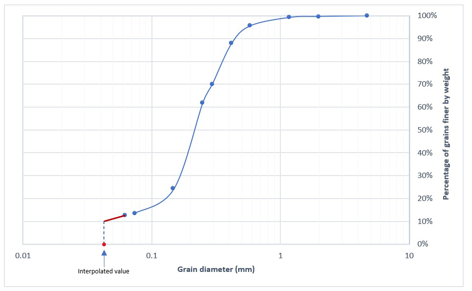
As mentioned before, the determination of grain size distribution for silt and clay (grains smaller than 0.075 mm), was performed when the percentage of fines was above 15%. In some cases that would imply that d₁₀ would be determined by interpolation, considering a straight line passing through the last two points of the grain-size distribution curve (Figure 5). That would not be a problem for methods that use d₂₀ or d₅₀ as effective grain size, notably Shepherd and USBR methods, but can add imprecision to the other methods. This was especially a concern for methods Kozeny-Carman and Therzaghi where an error of just 10% in the determination of d₁₀ would result in variations of the overall results by one order of magnitude. Another source of imprecision is the limited applicability of some methods since as mentioned before, not all methods apply to all points.

Figure 5
Grain size distribution curve and d₁₀ determination.

Average values and support volume

When the average value for each method is compared with the average of field measurements, the results are quite similar (Table 8).

Table 8
Average values of Ks for the watershed.

Method	Ks (cm/s)
Guelph	2.97x10-3
Shepherd	2.78x10-3
Hazen	3.10x10-3
Hazen Complete	4.27x10-3
Kozeny-Carman	4.36x10-3
Beyer	3.98x10-3
Slichter	1.45x10-3
Terzaghi	1.88x10-3
USBR	1.72x10-3

The PTFs with average results closest to field average measurements are the Shepherd and Hazen methods. The PTFs results separated by geological formations are given in Table 9.

Table 9
PTF results by geological formation.

Formation	Guelph	Shepherd	Hazen	Hazen C	Kozeny-Carman	Beyer	Slichter	Terzaghi	USBR
Piramboia	1.749x10-3	2.981x10-3	4.176x10-3	5.733x10-3	5.779x10-3	5.364x10-3	1.593x10-3	2.472x10-3	1.256x10-3
Botucatu	2.865x10-3	2.435x10-3	4.691x10-3	6.807x10-3	7.421x10-3	6.219x10-3	2.409x10-3	3.222x10-3	1.273x10-3
Serra Geral	8.850x10-4	4.470x10-6	7.812x10-7	7.819x10-7	5.542x10-7	8.609x10-7	2.099x10-7	4.501x10-7	4.522x10-8
Tertiary Deposits	1.110x10-3	3.362x10-3	5.258x10-3	5.096x10-4	3.377x10-4	5.680x10-4	1.316x10-4	1.763x10-4	1.036x10-4
Weighted average (area)	1.971x10-3	2.330x10-3	3.787x10-3	4.761x10-7	4.993x10-3	4.407x10-3	1.515x10-3	2.156x10-3	9.610x10-4

Computing K_s weighted average considering the area occupied by each formation in the sub-basin, PTF methods of Shepherd and Terzaghi have the best results when compared with field values (Table 9).

In general, the data is consistent considering the separation by geological units. The differences observed for the Serra Geral formation with Guelph permeameter, of at least two orders of magnitude, can be explained by the soil structure that can create a secondary porosity not captured by the PTF methods.

Despite the limited range of applicability for some of the PTF methods chosen, some of the results were remarkably similar for the study area. Engelbrecht et al. (2020), have chosen to use the Kozeny-Carman method to determine K_s of the GAS even though this method is more suitable for large-grain sands.

It is important to notice that PTF formulas developed using field data were often correlated with average K_s values from pumping tests. As the pumping test employs a large support volume, the respectively derived formulas are primarily valid for a general and not high-resolution aquifer characterization (Vienken & Dietrich, 2011).

Particle size is just one of the physical characteristics that influence hydraulic conductivity. The shape and arrangement of such particles, for instance, have a great influence on pore size distribution and connectivity. Point scale measurements cannot account for such variation, therefore several measurements across the area of interest are required to capture this variability. The volume of soil within which flow parameters are averaged and remain practically constant, is called a representative elementary volume (REV) (Lin & Rathbun, 2003). The REV is the scale at which the number of pore combinations is sufficient for variability to be considered stochastic and a single composite value can be used. Thus, all field-scale soil water models consider soil water variations due to individual particle interactions to be stochastic (Seyfried, 2003).

Despite collecting data across different formations and soil types, the granulometry of the samples as illustrated in Figure 2 is remarkably similar for almost all samples. Therefore, in this particular study, we are confident that the sampling distribution across the studied area captured the stochastic variation of K_s, and therefore, the average values obtained by field measurements and by most PTFs can be used as a composite K_s value for the referred watershed. We consider for the studied area that the best method is the Shepherd method, based on its range of applicability and results. It cannot be affirmed however that this number and distribution of sampling points can be used to obtain unique K_s values for watersheds of similar size and different soil conditions, for REV size vary greatly from place to place (Huang et al., 2016).

CONCLUSIONS

In this study PTFs proved to be a good surrogate to field measurement, provided that we use the average values of the sampling points, therefore fulfilling the objective of obtaining a composite K_s value for the catchment. For point estimates, that is, for higher spatial resolution, none of the PTF methods was adequate. The main limitations were related to the range of applicability of the PTFs, like for instance, grain size, level of uniformity, or abundance of the clay fraction. Therefore, in each case, a choice of the most compatible PTF should be made.

The results reinforce the viability of determining K_s using soil granulometry determination, which is a considerably cheaper, and less time-consuming task. However, it is important to notice that, as illustrated in Figure 2, in terms of granulometry, the area is quite homogeneous.

Further investigation is required to determine the minimum number of sampling points per catchment area, as well as if this method could be useful in catchments with more heterogeneous soil granulometry.

Associated Editor: Fernando Mainardi Fa

ACKNOWLEDGEMENTS

We want to thank the financial support of the National Council for Scientific and Technological Development (CNPq), through Project #404979/2018-1 and Scholarships #154684/2018-0; #800571/2016-9 and #134919/2019-0. We also want to thank the financial support from the São Paulo Research Foundation (FAPESP) through Grant Project #2018/0666-4 and scholarship #2019/03467-3.

REFERENCES

• Appels, W. M., Graham, C. B., Freer, J. E., & Mcdonnell, J. J. (2015). Factors affecting the spatial pattern of bedrock groundwater recharge at the hillslope scale. Hydrological Processes, 29(21), 4594-4610. http://dx.doi.org/10.1002/hyp.10481
  » http://dx.doi.org/10.1002/hyp.10481
• Ayers, J. F., Chen, X., & Gosselin, D. C. (1998). Behavior of nitrate-nitrogen movement around a pumping high-capacity well: a field example. Ground Water, 36(2), 325-337. http://dx.doi.org/10.1111/j.1745-6584.1998.tb01098.x
  » http://dx.doi.org/10.1111/j.1745-6584.1998.tb01098.x
• Batista, L. V., Gastmans, D., Sánchez-Murillo, R., Farinha, B. S., Dos Santos, S. M. R., & Kiang, C. H. (2018). Groundwater and surface water connectivity within the recharge area of Guarani aquifer system during El Niño 2014–2016. Hydrological Processes, 32(16), 2483-2495. http://dx.doi.org/10.1002/hyp.13211
  » http://dx.doi.org/10.1002/hyp.13211
• Bosch, D. D., & West, L. T. (2010). Hydraulic conductivity variability for two sandy soils. Soil Science Society of America Journal, 62(1), 90-98. http://dx.doi.org/10.2136/sssaj1998.03615995006200010012x
  » http://dx.doi.org/10.2136/sssaj1998.03615995006200010012x
• Brady, N. C., & Weil, R. R. (2014). Nature and properties of soils (14th ed.). London: Pearson.
• Cornelis, W. M., Ronsyn, J., van Meirvenne, M., & Hartmann, R. (2001). Evaluation of pedotransfer functions for predicting the soil moisture retention curve. Soil Science Society of America Journal, 65(3), 638-648. http://dx.doi.org/10.2136/sssaj2001.653638x
  » http://dx.doi.org/10.2136/sssaj2001.653638x
• De Pue, J., Rezaei, M., van Meirvenne, M., & Cornelis, W. M. (2019). The relevance of measuring saturated hydraulic conductivity: sensitivity analysis and functional evaluation. Journal of Hydrology, 576, 628-638. http://dx.doi.org/10.1016/j.jhydrol.2019.06.079
  » http://dx.doi.org/10.1016/j.jhydrol.2019.06.079
• Engelbrecht, B. Z., Teramoto, E. H., Gonçalves, R. D., & Chang, H. K. (2020). Hydraulic conductivity derived from geophysical logging in the Guarani Aquifer System. Holos Environment, 20(1), 117-136. http://dx.doi.org/10.14295/holos.v20i1.12369
  » http://dx.doi.org/10.14295/holos.v20i1.12369
• Fetter, C. W. (2014). Applied hydrogeology (4th ed.). Harlow: Pearson.
• Gastmans, D., Chang, H. K., & Hutcheon, I. (2010). Groundwater geochemical evolution in the northern portion of the Guarani Aquifer System (Brazil) and its relationship to diagenetic features. Applied Geochemistry, 25(1), 16-33. http://dx.doi.org/10.1016/j.apgeochem.2009.09.024
  » http://dx.doi.org/10.1016/j.apgeochem.2009.09.024
• Ghosh, B., & Pekkat, S. (2019). A critical evaluation of the variability induced by different mathematical equations on hydraulic conductivity determination using disc infiltrometer. Acta Geophysica, 63(3), 863-877. http://dx.doi.org/10.1007/s11600-019-00266-6
  » http://dx.doi.org/10.1007/s11600-019-00266-6
• Guzman, C. D., Hoyos-Villada, F., Da Silva, M., Zimale, F. A., Chirinda, N., Botero, C., Morales Vargas, A., Rivera, B., Moreno, P., & Steenhuis, T. S. (2019). Variability of soil surface characteristics in a mountainous watershed in Valle del Cauca, Colombia: implications for runoff, erosion, and conservation. Journal of Hydrology, 576, 273-286. http://dx.doi.org/10.1016/j.jhydrol.2019.06.002
  » http://dx.doi.org/10.1016/j.jhydrol.2019.06.002
• Huang, M., Zettl, J. D., Lee Barbour, S., & Pratt, D. (2016). Characterizing the spatial variability of the hydraulic conductivity of reclamation soils using air permeability. Geoderma, 262, 285-293. http://dx.doi.org/10.1016/j.geoderma.2015.08.014
  » http://dx.doi.org/10.1016/j.geoderma.2015.08.014
• Kanwar, R. S., Rizvi, H. A., Ahmed, M., Horton, R., & Marley, S. J. (1989). Measurement of field saturated hydraulic conductivity by using Guelph and Velocity permeameters. Transactions of the ASAE. American Society of Agricultural Engineers, 32(6), 1885-1890. http://dx.doi.org/10.13031/2013.31239
  » http://dx.doi.org/10.13031/2013.31239
• Kresic, N. (2007). Hydrogeology and groundwater modeling (2nd ed.). Boca Raton: CRC Press.
• Krueger, E. S., Ochsner, T. E., Engle, D. M., Carlson, J. D., Twidwell, D., & Fuhlendorf, S. D. (2015). Soil Moisture Affects Growing-Season Wildfire Size in the Southern Great Plains. Soil Science Society of America Journal, 79(6), 1567-1576. http://dx.doi.org/10.2136/sssaj2015.01.0041
  » http://dx.doi.org/10.2136/sssaj2015.01.0041
• Kutílek, M., & Nielsen, D. R. (1994). Soil hydrology Cremlingen: Catena Verlag.
• Lal, R., & Shukla, M. (2004). Principles of soil physics New York: Marcel Dekker. http://dx.doi.org/10.4324/9780203021231
  » http://dx.doi.org/10.4324/9780203021231
• Libohova, Z., Schoeneberger, P., Bowling, L. C., Owens, P. R., Wysocki, D., Wills, S., Williams, C. O., & Seybold, C. (2018). Soil systems for upscaling saturated hydraulic conductivity for hydrological modeling in the critical zone. Vadose Zone Journal, 17(1), 1-20. http://dx.doi.org/10.2136/vzj2017.03.0051
  » http://dx.doi.org/10.2136/vzj2017.03.0051
• Lin, H., & Rathbun, S. (2003). Hierarchical frameworks for multiscale bridging in hydropedology. In Y. A. Pachepsky, D. E. Radcliffe & H. M. Selim (Eds.), Scaling methods in soil physics (pp. 347-366). New York: CRC Press.
• Mbonimpa, M., Aubertin, M., Chapuis, R. P., & Bussière, B. (2002). Practical pedotransfer functions for estimating the saturated hydraulic conductivity. Geotechnical and Geological Engineering, 20(3), 235-259. http://dx.doi.org/10.1023/A:1016046214724
  » http://dx.doi.org/10.1023/A:1016046214724
• Mesquita, M., & Moraes, S. O. (2004). A dependência entre a condutividade hidráulica saturada e atributos físicos do solo. Ciência Rural, 34(3), 963-969. http://dx.doi.org/10.1590/S0103-84782004000300052
  » http://dx.doi.org/10.1590/S0103-84782004000300052
• Odong, J. (2007). Evaluation of empirical formulae for determination of hydraulic conductivity based on grain-size analyses. The Journal of American Science, 3, 54-60.
• Oliva, A., Hung Kiang, C., & Caetano-Chang, M. R. (2005). Determinação da condutividade hidráulica da Formação Rio Claro: análise comparativa através de análise granulométrica e ensaios com permeâmetro Guelph e testes de slug. Águas Subterrâneas, 19(2), 1-17.
• Organização dos Estados Americanos – OEA. (2009). Aquífero Guarani: programa estratégico de ação (424 p.). Washington: OEA.
• Rabelo, J. L., & Wendland, E. (2009). Assessment of groundwater recharge and water fluxes in the Guarani Aquifer System, Brazil. Hydrogeology Journal, 17(7), 1733-1748. http://dx.doi.org/10.1007/s10040-009-0462-y
  » http://dx.doi.org/10.1007/s10040-009-0462-y
• Radcliffe, D. E., & Simunek, J. (2010). Soil physics with hydrus Boca Raton: CRC Press.
• Reynolds, W. D., & Elrick, D. E. (1986). A method for simultaneous in situ measurement in the vadose zone of field‐saturated hydraulic conductivity, sorptivity, and the conductivity‐pressure head relationship. Groundwater Monitoring & Remediation, 6(1), 84-95. http://dx.doi.org/10.1111/j.1745-6592.1986.tb01229.x
  » http://dx.doi.org/10.1111/j.1745-6592.1986.tb01229.x
• Seyfried, M. S. (2003). Incorporation of remote sensing data in an upscaled soil water model. In Y. A. Pachepsky, D. E. Radcliffe & H. M. Selim (Eds.), Scaling methods in soil physics (417 p.). New York: CRC Press. http://dx.doi.org/10.1201/9780203011065.ch18
  » http://dx.doi.org/10.1201/9780203011065.ch18
• Sindico, F., Hirata, R., & Manganelli, A. (2018). The Guarani Aquifer System: from a Beacon of hope to a question mark in the governance of transboundary aquifers. Journal of Hydrology Regional Studies, 20, 49-59. http://dx.doi.org/10.1016/j.ejrh.2018.04.008
  » http://dx.doi.org/10.1016/j.ejrh.2018.04.008
• Soares, A. P., Soares, P. C., & Holz, M. (2008). Heterogeneidades hidroestratigráficas no Sistema Aqüífero Guarani. Revista Brasileira de Geociencias, 38(4), 598-617. http://dx.doi.org/10.25249/0375-7536.2008384598617
  » http://dx.doi.org/10.25249/0375-7536.2008384598617
• Song, J., Chen, X., Cheng, C., Wang, D., Lackey, S., & Xu, Z. (2009). Feasibility of grain-size analysis methods for determination of vertical hydraulic conductivity of streambeds. Journal of Hydrology, 375(3-4), 428-437. http://dx.doi.org/10.1016/j.jhydrol.2009.06.043
  » http://dx.doi.org/10.1016/j.jhydrol.2009.06.043
• Soto, M. A. A., & Kiang, C. H. (2018). Avaliação da condutividade hidráulica em dois usos do solo na região central do Brasil. Revista Brasileira de Ciências Ambientais, 47(47), 1-11. http://dx.doi.org/10.5327/Z2176-947820180169
  » http://dx.doi.org/10.5327/Z2176-947820180169
• Sperry, J. M., & Peirce, J. J. (1995). A model for estimating the hydraulic conductivity of granular material based on grain shape, grain size, and porosity. Ground Water, 33(6), 892-898. http://dx.doi.org/10.1111/j.1745-6584.1995.tb00033.x
  » http://dx.doi.org/10.1111/j.1745-6584.1995.tb00033.x
• Sprenger, M., Volkmann, T. H. M., Blume, T., & Weiler, M. (2015). Estimating flow and transport parameters in the unsaturated zone with pore water stable isotopes. Hydrology and Earth System Sciences, 19(6), 2617-2635. http://dx.doi.org/10.5194/hess-19-2617-2015
  » http://dx.doi.org/10.5194/hess-19-2617-2015
• Sracek, O., & Hirata, R. (2002). Geochemical and stable isotopic evolution of the Guarani Aquifer System in the state of São Paulo, Brazil. Hydrogeology Journal, 10(6), 643-655. http://dx.doi.org/10.1007/s10040-002-0222-8
  » http://dx.doi.org/10.1007/s10040-002-0222-8
• Tundisi, J. G., Matsumura-Tundisi, T., Pareschi, D. C., Luzia, A. P., Von Haeling, P. H., & Frollini, E. H. (2008). A bacia hidrográfica do tietê/Jacaré: estudo de caso em pesquisa e gerenciamento. Estudos Avançados, 22(63), 159-172. http://dx.doi.org/10.1590/S0103-40142008000200010
  » http://dx.doi.org/10.1590/S0103-40142008000200010
• U.S. Department of Agriculture – USDA. (2020). Soil texture calculator Washington: USDA. Retrieved in 2020, November 14, from https://www.nrcs.usda.gov/wps/portal/nrcs/detail/soils/survey/?cid=nrcs142p2_054167
  » https://www.nrcs.usda.gov/wps/portal/nrcs/detail/soils/survey/?cid=nrcs142p2_054167
• Vereecken, H., Weynants, M., Javaux, M., Pachepsky, Y., Schaap, M. G., & van Genuchten, M. T. (2010). Using pedotransfer functions to estimate the van Genuchten-Mualem soil hydraulic properties: a review. Vadose Zone Journal, 9(4), 795-820. http://dx.doi.org/10.2136/vzj2010.0045
  » http://dx.doi.org/10.2136/vzj2010.0045
• Vienken, T., & Dietrich, P. (2011). Field evaluation of methods for determining hydraulic conductivity from grain size data. Journal of Hydrology, 400(1-2), 58-71. http://dx.doi.org/10.1016/j.jhydrol.2011.01.022
  » http://dx.doi.org/10.1016/j.jhydrol.2011.01.022
• Willmott, C. J. (1981). On the validation of models. Physical Geography, 2(2), 184-194. http://dx.doi.org/10.1080/02723646.1981.10642213
  » http://dx.doi.org/10.1080/02723646.1981.10642213
• Zehe, E., Lee, H., & Sivapalan, M. (2006). Dynamical process upscaling for deriving catchment scale state variables and constitutive relations for meso-scale process models. Hydrology and Earth System Sciences, 10(6), 981-996. http://dx.doi.org/10.5194/hess-10-981-2006
  » http://dx.doi.org/10.5194/hess-10-981-2006
• Zhang, Y., & Schaap, M. G. (2019). Estimation of saturated hydraulic conductivity with pedotransfer functions: a review. Journal of Hydrology, 575, 1011-1030. http://dx.doi.org/10.1016/j.jhydrol.2019.05.058
  » http://dx.doi.org/10.1016/j.jhydrol.2019.05.058
• Zuquette, L. V., & Palma, J. B. (2006). Avaliação da condutividade hidráulica em área de recarga no aquífero Botucatu. Revista da Escola de Minas de Ouro Preto, 59(1), 81-87. http://dx.doi.org/10.1590/S0370-44672006000100011
  » http://dx.doi.org/10.1590/S0370-44672006000100011

Edited by

Editor-in-Chief: Adilson Pinheiro

Associated Editor: Fernando Mainardi Fa

Publication Dates

• Publication in this collection
  13 Dec 2021
• Date of issue
  2021

History

• Received
  30 Mar 2021
• Reviewed
  28 Sept 2021
• Accepted
  14 Oct 2021