SPEI and Hurst Analysis of Precipitation in the Amazonian Area of Brazil

SPEI e Análise de Hurst da Precipitação na área Amazônica do Brasil

Abstract

Amazon rainforest controls, to some extent, the global hydrological cycle. The objectives of the present work were (i) to investigate hydrologicalpatterns in a larger regionof the Brazilian rainforestthrough 9-month SPEI series and (ii) to search for long or short-term correlation within the number of days with precipitation by monthand accumulated monthly rainfall. Data sets were collected from 15 meteorological stations spanning a large area of the Amazonian rainforest in Brazil. We computed SPEI values from monthly precipitation and monthly meantemperature time series and determined Hurst exponents from detrendedtime series of days with precipitationand accumulated monthly rainfall. In the first case SPEI was determined on a 9-month timescale while Hurst exponents were calculated from rescaled range analysis. Percentage of SPEI values in the near normal class (-1 ≤SPEI ≤ 1) ranged from 59.8% (Peixe, TO) to 69.7% (Tarauaca, AC). The Hurst exponent varied from 0.382 (Diamantino, MT) to 0.636 (Tefé, AM) and correlated positively with the monthly meanrainfall. This indicates a persistenttrend of wet patterns in the futurein some areas. Hurst analysis of days with precipitation and monthly rainfallcould be an additional tool for interpreting rainfall data.

Keywords:
precipitation; spei; Hurst analysis; Amazonian rainforest

Resumo

A floresta amazônica controla, em certa medida, o ciclo hidrológico global. Os objetivos do presente trabalho foram (i) investigar padrões hidrológicos em uma área maior da floresta tropical brasileira por meio do SPEI baseado em 9-meses e (ii) buscar correlação de longo ou curto prazo dentro do número de dias com precipitaçãoe chuva mensal. Os conjuntos de dados foram coletados de 15 estações meteorológicas que abrangem uma grande área da floresta amazônica. Além disso, calculamos os valores de SPEI a partir de séries temporais mensais de precipitação e de temperatura media e determinamos os expoentes de Hurst a partir de séries temporais padronizadas de dias com precipitaçãoe séries mensais de precipitação. No primeiro caso, o SPEI foi determinado em uma escala temporal de 9 meses, enquanto os expoentes de Hurst foram calculados a partir da análise de escala re-escalonada. O percentual de valores de SPEI na classe normal variou de 59,8% (Peixe, TO) a 69,7% (Tarauaca, AC). O expoente de Hurst variou de 0,382 (Diamantino, MT) a 0,636 (Tefé, AM) e correlacionou-se positivamente com os dados de precipitação media. Isso indica uma tendência persistente de padrões úmidos no futuroem algumas áreas. A análise de Hurst de dias com precipitação e chuva mensalpode ser uma ferramenta adicional para interpretar dados de precipitação.

Palavras-chave:
precipitação; spei; análise de Hurst; floresta Amazônica

1.

Introduction

The Amazon rainforest is the largest ecosystem around the world. It controls, to some extent, the global hydrological cycle (Yoon and Zeng, 2010). In particular, Brazil holds the major part of that ecological reserve. The Amazon basinhas attracted a lot of investigations in terms of water balance, global carbon cycle or impact of climate change. It is considered one of the regions with strongest convective activity around the world (Andreoli et al. 2012). According to Marengo et al. (2004) precipitations in the Amazon have shown an unclear trend as multidecadal variations have presented opposite tendencies in the northern and southern areas of the basin. In particular, the time period 1950-1976 was wet in northern Amazonia and drier since 1976 (IPCC, 2001). In 2005, western Amazonia recorded its worst drought in 40 years (Zeng et al., 2008). Rainfall variability in Amazonia is correlated with the sea surface temperature (SST) patterns in the Atlantic and Pacific oceans during December, January and February (Martins et al., 2015). On the other hand, past investigations have shown a decadal intensification of rainfall over the whole Amazon basin (Chen et al., 2002).

In general, drought is very hard to define. Mishra and Singh (2010) have presented a review of drought concepts and its impact around the world during recent decades. Aragão et al. (2012) investigated the relationship between droughts and deforestation while Bonini et al. (2014) found significant negative correlations between deforestation and local precipitation in Mato Grosso, southern Brazil. Several statistical methods have been used for monitoring the severity of rainfall shortage. Palmer (1965) proposed the Palmer Drought Severity Index (PDSI) for characterization of meteorological drought. McKee et al. (1993) proposed the standardized precipitation index (SPI) to evaluate drought conditions for various timescales in different scenarios. Drought is usually grouped into meteorological drought (1- to 3- month timescale) to hydrological drought (6- month up to 24- month timescale) in terms of several indexes (Wildhite and Glantz, 1985). However, the main problem is that SPI is based on precipitation data only. This implies that SPI does not recognize the influence of temperature on drought conditions. More recently Vicente-Serrano et al. (2010) proposed the standardized precipitation evapotranspiration index (SPEI) which is based on precipitation and temperature (e.g. evapotranspiration) records. Tsakiris and Vangelis (2005) have stressed on the motivation for using potential evapotranspiration (PET) in drought severity evaluation. Those authors considered that PET can be considered as a key variable representing the intensity of the atmosphere to extract water from a selected system. Even thoughSPI and SPEI are valuable tools within the context of hydrological sciences, those indexes do not permit to detect hidden trends or to detect the probability of future extreme events. In this context, the rescaled range analysis (R/S) developed by Hurst (1951) to predict Nile River flooding could be a valuable tool for a better analysis and interpretation of SPEI time series. This nonlinearmethod has been used with rainfall data corresponding to several climatic environments (e.g. Zhou et al., 2005). While traditional drought indicators (e.g. SPI or SPEI) use one month or one week as the minimal timescale, R/S can analyze smaller timescales (e.g. minutes, hours or days) in terms of up- or down- scaling. Thus, our main hypothesis is that Hurst exponents computed from R/S analyses could be statistically correlated to SPEI values. The objectives of the present work were (i) to investigate hydrologicalpatterns in a larger region of the Brazilian rainforest through 9-month SPEI series and (ii) to search for long- or short-term correlation within the number of days with precipitation by monthand accumulated monthly rainfall.

2.

Material and Methods

2.1.

Study area and data characteristics

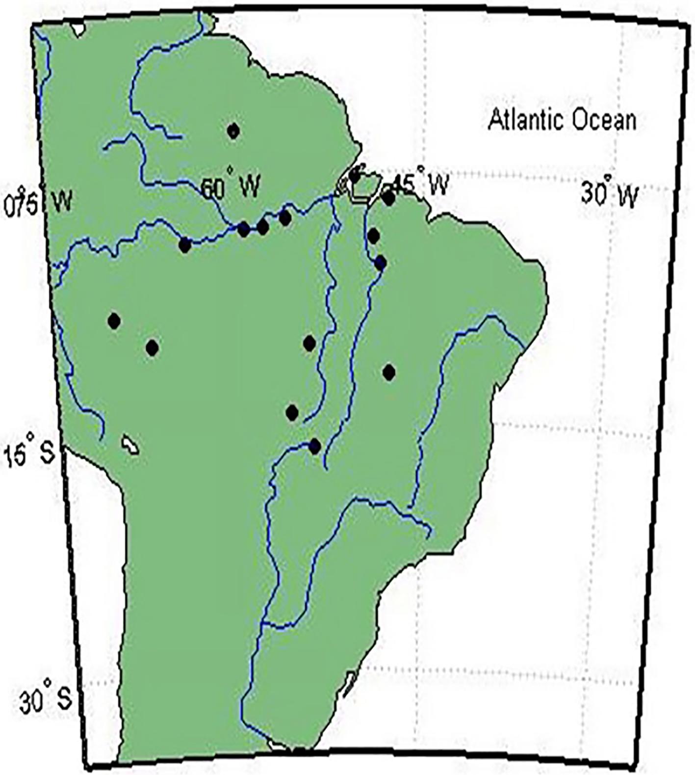
The study covers an important part of the Amazonian area of Brazil (e.g. from -48.35° to -70.76° West Longitude and -16.45° to 2.82° South Latitude). The spatial distribution of the meteorological stations is presented in Fig. 1. We considered a total of fifteen sites across seven Amazon states from Brazil. Table 1 shows basic information (e.g. geographical coordinates and height above sea level)about each meteorological station. We collected accumulated monthly rainfall and monthly mean temperature from each meteorological station. In order to investigate recent hydrometeorological patterns, we used uniform rainfall datasets ranging from 2001 to 2015. In addition, the number of days with precipitation by month for the same time period was also collected from each meteorological station.

Figure 1
Geographical location of meteorological stations.

Table 1.
General information of meteorological stations

Station ID	Location	State	Longitude (°)	Latitude (°)	h.a.s.l (m)*
82191	Belem	Pará	-48.43	-1.43	10.0
82024	Boa Vista	Roraima	-60.66	2.82	83.0
83309	Diamantino	Mato Grosso	-56.45	-14.4	286.3
82336	Itacoatiara	Amazonas	-58.43	-3.13	40.0
82098	Macapá	Amapá	-51.11	-0.05	14.46
82331	Manaus	Amazonas	-60.01	-3.1	61.25
82562	Marabá	Pará	-49.13	-5.36	95.0
83214	Matupá	Mato Grosso	-54.91	-10.25	285.0
82240	Parintins	Amazonas	-56.73	-2.63	29.0
83228	Peixe	Tocantins	-48.35	-12.01	242.49
82915	Rio Branco	Acre	-67.8	-9.96	160.0
83410	Rondonopolis	Mato Grosso	-54.56	-16.45	284.0
82807	Tarauaca	Acre	-70.76	-8.16	190.0
82317	Tefé	Amazonas	-64.7	-3.83	47.0
82361	Tucurui	Pará	-49.66	-3.76	40.0

• ^*
  height above sea level.

2.2.

Standardized Precipitation Evapotranspiration Index (SPEI)

Monthly rainfall and monthly mean temperature records were used for computing the standardized precipitation evapotranspiration index (SPEI) on a 9-month timescale. In particular, that timescale could be convenient for monitoring inter-seasonal hydrological patterns (WMO, 2012). The mathematical rationale of SPEI is well described in Vicente-Serrano et al. (2010). However, we describe here its basic grounds:

Basically, the SPEI makes use of the difference between the monthly or weekly precipitation (P) and potential evapotranspiration (PET). The PET values are computed following the approach by Thornthwaite (1948). That is, the monthly PET (mm) is calculated as:

(1) $$PET=16K{\left(\frac{10T}{I}\right)}^m$$

where T is the monthly mean temperature (°C), I, is a heat index which is the sum of 12 monthly index values, i:

(2) $$i={\left(\frac{T}{5}\right)}^{1.514}$$

(3) $$m=6.75\times {10}^{-7}{I}^3-7.71\times {10}^{-5}{I}^2+1.79\times {10}^{-2}I+0.492$$

and K is a correction factor computed as a function of the month and latitude.

(4) $$K=\left(\frac{N}{12}\right)\left(\frac{NDM}{30}\right)$$

NDM is the number of days of the month and N is the maximum number of sun hours.

(5) $$N=\left(\frac{24}{\pi }\right){\omega }_s$$

where ω_s is the hourly angle of sun rising.

(6) $${\omega }_s=\arccos \left(-tan\phi tan\delta \right)$$

Here φ is the latitude in radians and δ is the solar declination in radians.

(7) $$\delta =0.4093sen\left(\frac{2\pi J}{365}-1.405\right)$$

where J is the average Julian day of the month.

The difference between rainfall P and PET for the i -month, is computed as:

(8) $$D_i=P_i-PE{T}_i$$

The computed D_iv values are then aggregated at different timescales in the same way as that for computing SPI. That is, the difference D in a given month j and year i depends on the timescale k (e.g. 1, 3, 6,.., 24 months). We reproduce here the same example used by Vicente-Serrano et al. (2010). For instance, the accumulated difference for one month in a particular year i with a 12-month timescale is calculated as:

(9) $$X_{i,j}^k={\displaystyle {\sum }_{l=13-k+j}^{12}\left({\text{D}}_{\text{i}-1,\text{l}}\right)}+{\displaystyle {\sum }_{l=1}^j\left({\text{D}}_{\text{i},\text{l}}\right)},\text{if j}<k$$

and:

(10) $$X_{i,j}^k={\displaystyle {\sum }_{l=j-k+1}^j\left({\text{D}}_{\text{i},\text{l}}\right)},\text{if j}\ge k$$

Here, D_i,l = P – PET in the first month of the year i in millimeters.

Different to SPI computation which uses a two parameter distribution (Gamma distribution), SPEI calculation requires a three-parameter distribution to model D_i values for different timescales. In this case, Vicente-Serrano et al. (2010) proposed a log-logistic distribution function. It is instructive to recall here that its probability density function is:

(11) $$f\left(x\right)=\frac{\beta }{\alpha }{\left(\frac{x-\gamma }{\alpha }\right)}^{\beta -1}{\left[1+{\left(\frac{x-\gamma }{\alpha }\right)}^{\beta }\right]}^{-2}$$

while its probability distribution function is:

(12) $$F\left(x\right)={\left[1+{\left(\frac{\alpha }{x-\gamma }\right)}^{\beta }\right]}^{-1}$$

where α, β, and γ are the scale, shape, and origin parameters, respectively.

After that, the SPEI can be calculated as standardized values of F(x):

(13) $$SPEI=W-\frac{C_0+C_{1}W+C_2{W}^2}{1+d_{1}W+d_2{W}^2+d_3{W}^3},\mathrm{where}W=\sqrt{-2\ln \left(p\right)},\mathrm{for}p\le 0.5$$

where p is the probability of exceeding a given D value, p= 1 – F(x), C₀ = 2.515517, C₁ = 0.802853, C₂= 0.010328, d₁ = 1.432788, d₂ = 0.189269, d₃= 0.001308. In addition, when p >0.5, it is replace by 1 – p and the sign of the corresponding SPEI value is inverted. The software for computing the SPEI isof public domain (Begueria and Vicente-Serrano, 2013).

2.3.

Rescaled range (R/S) analysis and Hurst exponent estimation

Each time series corresponding to the number of days with precipitation by month and accumulated monthly rainfall was detrended for removing trend and any seasonal component (Shumway and Stoffer, 2006). Furthermore, Mandelbrot and Wallis (1969) recommended removing periodic structures before the application of the R/S method:

(14) $$Y_{di}=Y_i-\left(a+b{t}_i\right)$$

where Y_di. is the ith detrended value at the i th month (t_i), Y_i is the ith observed (untransformed) record and a and b are the coefficients of the linear trend equation. This procedure transforms the original data into a residual time series. Thedetrended time series of days with precipitation by month were used for performing rescaled range (R/S) analysis and to compute the Hurst exponent (H_d hereafter) (Hurst, 1951). In addition, Hurst exponents were also computed from each time series corresponding to the accumulated monthly rainfall (H_r hereafter). The mathematical basis of the rescaled range method is described in many papers (e.g. Hurst, 1951; Feder, 1988; Turcotte, 1997; Shi et al., 2013). Nevertheless, it could beuseful to recall here its fundamentals:

Assume a time series of a given meteorological variable {Y (τ)} (τ = 1,2,…,m) and compute the mean value:

(15) $$Y_{\tau }=\frac{1}{\tau }{\displaystyle {\sum }_{t=1}^{\tau }Y\left(t\right)}$$

After that we calculate the cumulative deviation as:

(16) $$Y_{t,\tau }={\displaystyle {\sum }_{t=1}^{\tau }[Y\left(t\right)-Y_{\tau }],1\le t\le \tau }$$

Define a range series:

(17) $$R\left(\tau \right)=\begin{array}{l}maxY\left(t,\tau \right)-\\ 1\le t\le \tau \end{array}\begin{array}{l}minY\left(t,\tau \right)\\ 1\le t\le \tau \end{array}$$

The standard deviation series is defined as:

(18) $$S(\tau )=\sqrt{\left(\frac{1}{\tau }{{\displaystyle {\sum }_{t=1}^{\tau }[Y\left(t\right)-Y_{\tau }]}}^2\right)}$$

Finally, the rescaled range (R/S) is a power law of the time lag (τ):

(19) $${\left(R/S\right)}_{\tau }=c{\tau }^H$$

where H is the Hurst exponent (0 < H < 1) and c is a constant representing the rescaled range at a unit time scale (e.g. τ = one day). In practice, c and H are dependent constants.

Eq. (19) can be used with empirical or simulated observations after a log-log transformation:

(20) $$\log {\left[R/S\right]}_{\tau }=\log \left(c\right)+H\log \left(\tau \right)$$

The value of the Hurst exponent can be used to predict the future trend of a meteorological variable based on its current behavior. For example:

1. H = 0.5 indicates that rainfall variance is due to independent, random (Gaussian) processes. That is, there is no correlation between past and future rainfall events.

2. 0.5 < H < 1 signifies that past and future rainfall events are positively correlated. This positive trend (persistence) can span several time scales.

3. 0 < H < 0.5 implies that past and future rainfall events are negatively correlated in time. Such a negative trend (antipersistence) can also span several time scales.

The Hurst exponents estimated from the detrended number of days with precipitation by months are represented by H_d while those computed from monthly rainfall are denoted by H_r.

All the statistical analyses were conducted using StatisticaTM Software Package (StatSoft Inc., 2011).

3.

Results and Discussion

Table 2 shows the descriptive statistics of monthly rainfall corresponding to the whole available time period for each meteorological station. That classical analysis revealed a large spatio-temporal variability in terms of coefficient of variation (CV). It ranged from CV = 50.7% for Tefé (Amazonas state) to CV = 103% for Peixe (To­cantins state). The maximum precipitation values were registered in the Northern-Northeastern parts of the basin. For example, Parintins (Amazonas state) recorded 773.3 mm while Belem (Pará state) registered 742.5 mm. Note however that 9 out of 15 sites recorded months with zero rainfall. In general this information agrees, to some extent, with the mechanism of moisture transport and convergence evaluated by many simulation models (Martins et al., 2015). On the other hand, Table 3 presents the descriptive statistics of monthly mean temperature for all the sites. Mean temperature showed less variability as compared to precipitation in terms of CV values. Coefficient of variation (CV) spanned from 2.2% for Belem (Pa­rá state) to 6.3% for Rondonopolis (Mato Grosso state). Figure 2 presents the time series corresponding to monthly rainfall and monthly mean temperature for three selected sites (Boa Vista, Rondonopolis and Tefé). We found a slight increase of monthly mean temperature as shown by the trend line. For example, an increase of 0.47 °C was detected in Boa Vista (Roraima state), 0.70 °C in Rondonopolis (Mato Grosso state) and 0.31 °C in Tefé (Amazonas state. A similar trend was found for all the investigated time series. In the present study, the mean value of temperature increase was 0.71 °C for the 15 studied locations. This is consistent with the fact that, at a global scale, mean temperature has increased about 0.6 °C over the last century (Molla et al., 2006). According to an IPCC report (IPCC, 2007), an increasing rate of warming has occurred over the last 25 years.

Figure 2
Accumulated monthly rainfall and mean monthly temperature for three selected locations.

Table 2.
Descriptive statistics of monthly rainfall

Location	Mean (mm)	Min.(mm)	Max.(mm)	St. Dev.(mm)	CV(%)
Belem	278.3	41.3	742.5	155.7	56.0
Boa Vista	151.7	0.0	667.5	147.5	97.2
Diamantino	165.3	0.0	638.3	148.2	89.5
Itacoatiara	213.7	1.4	605.0	143.5	67.1
Macapá	207.8	0.0	679.2	155.9	75.0
Manaus	196.3	0.6	553.0	131.0	66.7
Marabá	148.9	0.0	517.8	132.5	88.9
Matupá	175.4	0.0	587.5	155.1	88.4
Parintins	220.1	1.3	773.3	162.2	73.7
Peixe	118.7	0.0	527.5	122.6	103
Rio Branco	164.5	0.0	512.2	116.5	70.8
Rondonopolis	108.0	0.0	572.2	110.4	102
Tarauaca	192.7	2.0	513.2	115.5	59.9
Tefé	210.7	26.0	637.2	106.8	50.7
Tucurui	206.2	0.0	732.3	178.5	86.5

Table 3.
Descriptive statistics of monthly mean temperature.

Location	Mean (°C)	Min.(°C)	Max.(°C)	St. Dev.(°C)	CV(%)
Belem	26.9	25.5	28.1	0.59	2.2
Boa Vista	28.1	25.7	30.1	0.95	3.4
Diamantino	25.3	21.3	28.3	1.47	5.8
Itacoatiara	27.3	22.8	30.1	1.00	3.6
Macapá	27.4	25.3	29.3	0.98	3.6
Manaus	27.4	25.2	30.2	1.00	3.6
Marabá	27.7	25.8	29.8	0.92	3.3
Matupá	25.4	23.7	27.7	0.76	3.0
Parintins	27.9	25.2	30.1	1.06	3.8
Peixe	26.2	22.9	29.0	1.15	4.4
Rio Branco	25.2	19.8	26.9	1.06	4.2
Rondonopolis	25.2	21.0	28.7	1.60	6.3
Tarauaca	25.8	20.3	27.2	0.81	3.2
Tefé	27.0	24.9	28.9	0.66	2.4
Tucurui	27.7	26.0	29.7	0.75	2.7

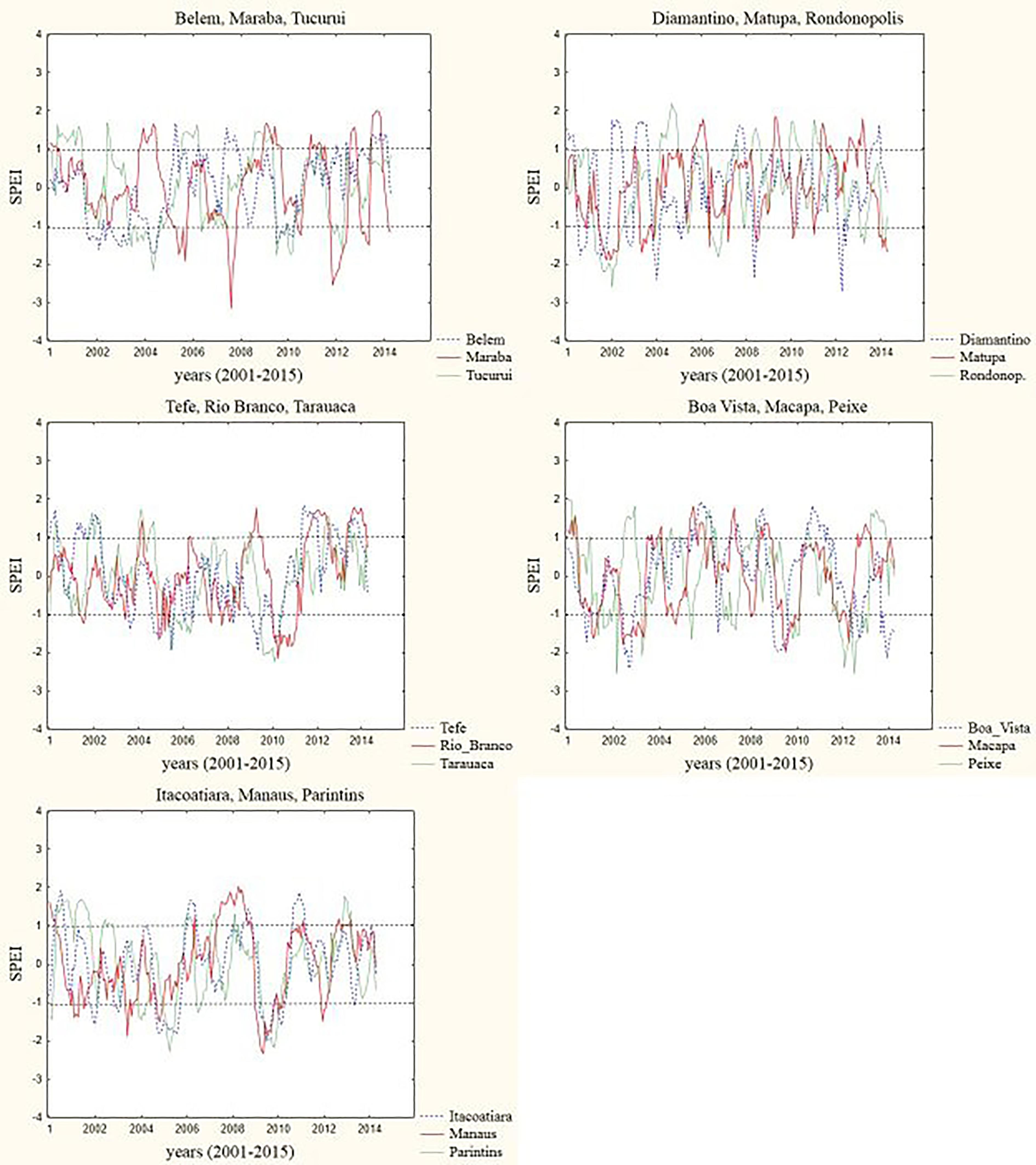
Figure 3 shows the SPEI oscillation for all the investigated locations. The percentage of SPEI values in the nearnormal class (-1 ≤ SPEI ≤ 1) ranged from a minimum 59.8% for Peixe (Tocantins state) to a maximum value 69.7% for Tarauaca (Acre state) (Table 4). On the other hand, the proportion of SPEI values within the moderate to extremely dry category (-3 ≤ SPEI < -1) ranged from 14.5% for Diamantino (Mato Grosso state) to 21.5% for Peixe(Tocantins state) (Table 4). In particular, we found important moderate to extreme droughtperiodsfor five investigated sites (e.g. a run of more than 12 consecutive months with SPEI < -1) (Fig. 3): for example Matupá (Mato Grosso state) approximately from May 2001 to April 2003 and Rondonopolis (Mato Grosso state) from March 2001 to June 2003. This is significant as Mato Grosso is located within the so-called deforestation arc (Bonini et al., 2014). One site from Amazonas state also showed more than 12 months of moderate to extreme drought: Itacoatiara (from August 2005 to October 2006. The longer period of moderate to extreme drought was detected for Peixe (Tocantins state) and lasted approximately 16 months (from March 2013 to October 2014) while Rio Branco (Acre state) showed a 14-month period of moderate to extreme dry (from March/April 2011 to May 2012 approximately). That residence time is more than 8% of the time within drought categories. Many authors have identified deforestation as the main cause of such a hydrological alteration (Moraes et al., 2013) whileother authors hold that drought is a multi-causal phenomenon (Zeng et al., 2008). Based on SPEI classification, the 9-month timescale detected hydrological drought in different regions of the Amazon basin spanning different periods of time. It could be useful to consider other SPEI time scales in the future. Note however, that SPEI values based on a single 9-month timescale detected drought periods unobserved in other studies. It is due, in part, to the insertion of mean temperature into the computations. We are well aware that availability of large precipitation and temperature records can improve the SPEI interpretation. However, we considered that the derived information for the last 15 years could be valuable within the context of the present investigation.

Figure 3
SPEI (9-month timescale) oscillation for all the investigated sites.

Table 4.
Percentage of SPEI values in approximately normal (-1 ≤SPEI ≤ 1) and moderate to extremely dry (-3≤ SPEI <-1) classes.

Location	-1 ≤SPEI ≤1 (%)	(-3≤SPEI <-1)
Belem	68.0	18.0
Boa Vista	65.6	16.8
Diamantino	67.7	14.5
Itacoatiara	65.0	20.3
Macapá	61.0	20.9
Manaus	65.1	16.8
Marabá	61.7	15.2
Matupá	66.8	18.0
Parintins	62.7	16.2
Peixe	59.8	21.5
Rio Branco	65.1	16.4
Rondonopolis	62.7	19.2
Tarauaca	69.7	15.7
Tefé	62.2	16.2
Tucurui	60.4	18.6

The Hurst exponent estimated from the detrended number of days with precipitation by month ranged from H_d = 0.382 (strong antipersistence) for Diamantino (Mato Grosso) to H_d = 0.636 (strong persistence) for Tefé (Amazonas) (Table 5). Based on the confidence limits of H_d estimates, those time series corresponding to Macapá (Amapá state), Marabá (Pará state), Matupá (Mato Grosso), Rio Branco (Acre state) and Tarauaca (Acre state) were very close to the theoretical Gaussian limit H_d= 0.5 (H_d = 0.533±0.017, H_d = 0.530±0.020, H_d= 0.468±0.022, H_d = 0.525±0.027 and H_d = 0.490±0.022, respectively). That is, at a first criterion we could accept the hypothesis on the independence (e.g. random increments) between past and future daily rainfall patterns. This suggests, to some extent, that those variables close connected to daily rainfall patterns such as air temperature, atmospheric moisture distribution or convective processes also could show random (Gaussian) variability in those particular sites (Fraedrich, 2002). In particular, H_d > 0.5 indicates that present and future daily rainfall patterns tend to persist, at least, in the near future. Some sites located at Central to Northeast Amazonia showed moderated persistence in the monthly number of days with rainfall occurrence (e.g. Belem, Manaus, Parintins) while some zones located at South to Southwest Amazonia presented moderated anti-persistence (e.g. Peixe, Rondonopolis) (Table 5). In this case, the observed daily rainfall patterns show a reversal trend. Hurst exponents estimated from detrended time series of accumulated monthly rainfall ranged from H_r = 0.302 for Peixe (Tocantins state) to H_r = 0.548 for Tefé (Amazonas state). Note that most H_r values were consistently below 0.5 (Table 5). We found a significant linear relationship (significance level p < 0.05) between Hurst exponents estimated from the number of days with precipitation by month (H_d) and monthly mean rainfall (Fig. 4):

Figure 4
Linear relationship between Hurst exponent (H_d) and the logarithm ofthe accumulated monthly rainfall.

Table 5.
Rescaled range analysis parameters[in parenthesis lower (-) and upper (+) confidence limits for a level α = 0.05].

Location	cd	Hd (days with rainfall)	R *		cr	Hr (monthly rainfall)	R *
Belem	1.60(±0.16)	0.552(±0.015)	0.950		1.56(±0.031)	0.409(±0.016)	0.965
Boa Vista	1.73(±0.17)	0.425(±0.014)	0.954		1.37(±0.028)	0.451(±0.014)	0.976
Diamantino	1.81(±0.14)	0.382(±0.021)	0.979		2.03(±0.038)	0.315(±0.020)	0.950
Itacoatiara	1.68(±0.08)	0.543(±0.014)	0.993		1.74(±0.047)	0.413(±0.025)	0.981
Macapá	1.70(±0.20)	0.533(±0.017)	0.910		1.61(±0.032)	0.405(±0.017)	0.963
Manaus	1.53(±0.16)	0.566(±0.018)	0.951		1.43(±0.029)	0.439(±0.015)	0.983
Marabá	1.69(±0.20)	0.530(±0.020)	0.950		1.78(±0.036)	0.382(±0.019)	0.950
Matupá	1.71(±0.16)	0.468(±0.022)	0.954		2.10(±0.042)	0.305(±0.022)	0.931
Parintins	1.54(±0.09)	0.567(±0.015)	0.991		1.46(±0.031)	0.434(±0.016)	0.970
Peixe	1.72(±0.10)	0.428(±0.027)	0.986		2.08(±0.042)	0.302(±0.022)	0.942
Rio Branco	1.71(±0.12)	0.525(±0.027)	0.976		1.70(±0.034)	0.379(±0.018)	0.957
Rondonopolis	1.72(±0.17)	0.430(±0.021)	0.912		1.25(±0.025)	0.469(±0.013)	0.989
Tarauaca	1.73(±0.10)	0.490(±0.022)	0.985		1.47(±0.029)	0.442(±0.015)	0.973
Tefé	1.46(±0.14)	0.636(±0.013)	0.958		0.96(±0.029)	0.548(±0.015)	0.982
Tucurui	1.68(±0.16)	0.544(±0.02)	0.950		1.65(±0.032)	0.400(±0.017)	0.961

• ^*
  Correlation coefficient.

(21) $$H_d=0.44\left(0.13\right)\log \left(P_{mean}\right)-0.485\left(0.29\right),R=0.793$$

where log(P_mean) is the logarithm of mean rainfall values as shown in Table 2.

Eq. (21) conveys information on the potential utility of Hurst analysis. Irrespective of the amount of daily rainfall, the scale invariance of detrendednumber of dayswith precipitation by month determines the randomness, persistence or anti-persistence of rainy patterns as a whole. It also suggests thatmoving from anti-persistence to persistence as a function of daily rainfall could be related toother scaling processes showingnegative correlation and trend reversal or positive correlation between past and present wet states and non-periodic cyclical pattern. For example, a typical case is the evaporation to precipitation ratio (Millán et al., 2009). In particular, the long-term memory effect could be induced by low frequency atmospheric variability (Fraedrich, 2003). For example, Manabe and Delworth (1990) considered that soil moisture can contribute to such low frequency atmospheric variability. The extreme cases of anti-persistence in terms of H value were found for Diamantino (H_d = 0.382 and H_r = 0.315) and Peixe (H_d = 0.428 and H_r = 0.302). This indicates that actual dry patterns detected in that zonescanintensify in the future so as the probability of extreme events (e.g. droughts). For example,Diamantino showed a rainfall decrease of about -12 mm while Tefé (H_d = 0.636 and H_r = 0.548) presented an increase of approximately +19 mm in the last 15 years. That information can be obtained from the linear trend of the original, untransformed, time series. In meteorological terms, few days with intense, local and short-lived rainfall events (e.g. convective rainfall events) in a month can produce a larger accumulated monthly rainfall than many days with stratiform rainfall. On this basis, we could hypothesize that H_d > 0.5 and H_r < 0.5 indicate that persistence of the number of days with precipitation by month combined with anti-persistence of the accumulated monthly rainfall are due to the relevance of stratiform rainfall more than convective rainfall(e.g. Belem, Tucurui) (Table 5). Thatassumption agrees with previous results derived from wavelet analysis by Venugopal and Foufoula-Georgiou (1996). Wang et al. (2010), using detrended fluctuation analysis, alsofound short-range and long-range correlations for the Amazon. Those authors also considered soil moisture as an important driving agent in land-atmosphere interactions. In particular, Mato Grosso showed a forest loss of about 13.4% in the period 2001-2012. That is, deforestation can intensify evaporation and soil moisture shortage. In fact, soil moisture deficit combined with high temperature affects evapotranspiration which also influences SPEI values. This could alsoexplain, to some extent, the anti-persistent rainfall patterns in some studied sites. Furthermore, evaporation can exceed precipitation in those deforested areas which could modify the hydrological cycle (Millán et al., 2009). We do not have any information on previous works relating scaling indexes as derived from fractal concepts to first order statistics (e.g. mean values) of hydrometeorological variables. SPEI and Hurst exponents are valuable parameters for identifying vulnerable areas in terms of extreme events (e.g. droughts and intense rainfall). It is also interesting that orographic factors (e.g. height above sea level) can also determine the nonlinear scaling of rainfall events. If one correlates the height above sea level (Table 1) with H_d (Table 5) will find a significant negative linear relationship between both parameters (R = -0.776, p < 0.05). This result is physically sound since one could expect a drier atmosphere as the height above sea level increases. Finally, we could identify two potential utilities of Hurst exponents for conducting hydrometeorological investigationsin the Amazon basin. First of all, H values can be incorporated within nonlinear models for making rainfall events simulation and second, the existence of scale invariance as represented by Hurst exponents is a key component for up-scaling atmospheric processes. That is, yearly rainfall dynamics could be modeled by actual monthly patterns.

4.

Conclusion

We used a 9-month timescalestandardized precipitation evapotranspiration index (SPEI) for investigating the current state of hydrometeorology in 15 sites of the Amazonian rainforest. Even thought the percentage of SPEI values within the near normal class was over59%, five sites showedmore than 12 consecutive months of moderate to extreme drought (-3 ≤ SPEI < -1). Hydrological droughts were present in different years within the considered time periodaccording to SPEI classification. In addition, we performed re-scaled range analysis (R/S) for estimating the Hurts exponent corresponding to each detrended time series of days with precipitation by month and monthly rainfall. There was a positive linear relationship between the Hurst exponent (H_d) and the monthly mean rainfall. This could help to incorporate theoretical concepts of scaling for interpreting the evolution in time ofrainfall events. As Amazonia climate is very complex, future investigations could be conducted to test whether persistence (H > 0.5) or anti-persistence (H < 0.5) of rainfall time series detected at smaller timescales (e.g. days) could be replicated at larger timescales (e.g. months or year. This would require larger data sets. Hurst exponents could be also associated to the rainfall generating mechanism (e.g. convective or stratiform rainfall). In terms of H_d and H_r, different Amazonian regions showed different rainfall regimes. That is, moderate persistence at Central to Northeast Amazonia to moderate anti-persistence at South to Southwest Amazonia with extreme cases at Mato Grosso state.

Acknowledgments

The authors want to acknowledge Instituto Nacional de Meteorologia (INMET, Brazil) for providing access to the rainfall and temperature data sets used in the present study. Dr. Humberto Millán is grateful to the Universidade do Estado do Amazonas (Manaus, Brazil) for the valuable support during his position as an invited Professor of Physics. Jakeline Rabelo Lima was supported by the FAPEAM Program (Fundação de Amparo á Pesquisa do Estado do Amazonas) under grant 22/2013-GR/UEA.

References

• ANDREOLI, R.V.; SOUSA, R.A.F.; KAYANO, M.T.; CANDIDO, L.A. Seasonal anomalous rainfall in the central and eastern Amazon and associated anomalous oceanic and atmospheric patterns. International Journal of Climatology, v. 32, p. 1193-1205, 2012
• ARAGãO, L.E.O.C.; MALHI, Y.; BARBIER, N.; LIMA, A.; SHIMABUKURU, Y.; ANDERSON, L.; SAATCHI, S. Interactions between rainfall, deforestation and fires during recent years in the Brazilian Amazonia. Philosophical Transactions of the Royal Society B, London, v.363, n. 1498, p. 1779-1785, 2012
• BEGUERIA, S.; VICENTE-SERRANO, S.M. Calculation of the standardized precipitation-evapotranspiration index. User manual, version 1.6, 16 p., available at http://sac.csic.es/spei, 2013
  » http://sac.csic.es/spei
• BONINI, I.; RODRIGUES, C.; DALLACORT, R.; JUNIOR, B.H.M.; CARVALHO, M.A.C. Rainfall and deforestation in the municipality of Colíder, southern Amazon. Revista Brasileira de Meteorologia, v.29, n.4, p. 483-493, 2014
• CHEN, J.; CARLSON, B.E.; DEL GENIO, A.D. Evidence for strengthening of the tropical circulation in the 1990s. Science, v. 295, p. 838-841, 2002
• FEDER, J. Fractals 2nd ed. Plenum Press, New York, 283p., 1988
• FRAEDRICH, K. Fickian diffusion and Newtonian cooling: A concept for noise induced climate variability with long-term memory?. Stochastics and Dynamics, v. 2, n. 3, p. 403-412, 2002
• FRAEDRICH, K. Predictability: short- and long-term memory of the atmosphere. In Boffetta, G., Lacorata, G., Visconti, G., Vulpiani, A. (eds.), Chaos in Geophysical Flows, International Summer School on Atmospheric and Oceanic Sciences, L’Aquila, Italy, p. 63-104, 2003
• HURST, H.E. Long-term storage capacity of reservoirs. Transactions of the American Society of Civil Engineering, v.116, p. 770-799, 1951
• INTERGOVERNMENTAL PANEL ON CLIMATE CHANGE. Climate Change 2001: Impacts, Adaptation, and Vulne­rability. Contribution of Working Group II to the Third Assessment Report of the Intergovernmental Panel on Climate Change Cambridge University Press, Cambridge , United Kingdom, 1032 p., 2001
• INTERGOVERNMENTAL PANEL ON CLIMATE CHANGE. Climate change 2007: The Physical Science Basics. In Solomon, S., Qin, D., Manning, M., Chen, Z., Marquis, M., Averyt, K.B., Tignor, M., Miller, H.L. (eds.), Contribution of Working Group I to the Fourth Assessment Report of the Intergovernmental Panel on Climate Change, Cambridge University Press, Cambridge, United Kingdom and New York, NY, USA, 996 p., 2007.
• MANABE, S.; DELWORTH, T. The temporal variability of soil wetness and its impact on climate, Climate Change, v. 16, p. 185-192, 1990
• MANDELBROT, B.B; WALLIS, J.R. Some long-run properties of geophysical records. Water Resources Research, v. 5, p. 242-259, 1969
• MARENGO, J. Interdecadal variability and trends of rainfall across the Amazonian basin. Theoretical and Applied Climatology, v.78, p. 79-96, 2004
• MARTINS, G.; VON RANDOW, C.; SAMPAIO, G.; DOLMAN, A.J. Precipitation in the Amazon and its relationship with moisture transport and tropical Pacific and Atlantic SST from the CMIP5 simulation. Hydrology and Earth System Sciences (Discussions), v. 12, p. 671-704, 2015
• McKEE, T.B.; DOESKEN, N.J.; KLEIST, J. The relationship of drought frequency and duration to time scales. Preprints, 8^th Conference on Applied Climatology, 17-22 January, American Meteorological Society, Anaheim, CA, p.179-184, 1993
• MILLáN, H.; KALAUZI, A.; LLERENA, G.; SUCOSHAñAY, J.; PIEDRA, D. Meteorological complexity in the Amazonian area of Ecuador: An approach based on dynamical system theory. Ecological Complexity, v. 6, p. 278-285, 2009
• MISHRA, A.K., SINGH, V.P. A review of drought concepts. Journal of Hydrology, v. 391, p. 202-216, 2010
• MOLLA, M.D.K.I.; RAHMAN, M.S.; SUMI, A.; BANIK, P. Empirical mode decomposition analysis of climate changes with special reference to rainfall data. Discrete Dynamics in Nature and Society, v. 2006, p. 1-17, 2006
• MORAES, E.C.; FRANCHITO, S.H.; RAO, V.B. Amazonian deforestation: impact of global warming on the energy ba­lance and climate. Journal of Applied Meteorology and Climatology, v. 52, n. 3, p. 521-530, 2013
• PALMER, W. Meteorological Drought. Research Paper 45, US Weather Bureau, Washington, D. C., 1965
• SHI, P.; MA, X.; CHEN, X.; QU, S.; ZHANG, Z. Analysis of variation trends in precipitation in an upstream catchment of Huai river. Mathematical Problems in Engineering, v. 2013, p. 1-11, 2013
• SHUMWAY, R.H; STOFFER, D.S. Time Series Analysis and Its Applications 2nd ed. Springer Science+Business Media, 588 p., 2006
• STATSOFT, INC. Statistica (Data Analysis Software System), version 10, Tulsa, OK, 2011
• THORNTHWAITE, C.W. An approach toward a rational classification of climate. Geographical Review, v. 38, p. 55-94, 1948
• TSAKIRIS, T.; VANGELIS, H. Establishing a drought index incorporating evapotranspiration. European Water, v. 9/10, p. 3-11, 2005
• TURCOTTE, D.L. Fractals and Chaos in Geology and Geophysics 2nd ed. Cambridge University Press, 412 p., 1997
• VENUGOPAL, V.; FOUFOULA-GEORGIOU, E. Time-frequency-scale analysis of high resolution temporal rainfall using wavelet packets. Journal of Hydrology, v. 187, p. 3-27, 1996
• VICENTE-SERRANO, S.M.; BEGUERíA, S.; LóPEZ-MO­RENO, J.I. A multiscalar drought index sensitive to global warming: The Standardized Precipitation Evapotranspiration Index. Journal of Climate, v.23, n.7, p.1696-1718, 2010
• WANG, G.; DOLMAN, A.J.; BLENDER, R.; FRAEDRICH, K. Fluctuation regimes of soil moisture in ERA-40 re-analysis data. Theoretical and Applied Climatology, v. 99, p. 1-8, 2010
• WILDHITE, D.A.; GLANTZ, M.H. Understanding the drought phenomenon: The role of definitions. Water International Journal, v.10, p. 111-120, 1985
• WORLD METEOROLOGICAL ORGANIZATION. Standardized Precipitation Index User Guide. World Meteorological Organization, n. 1090, 2012
• YOON, J.H.; ZENG, N. An Atlantic influence on Amazon rainfall. Climate Dynamics, v. 34, p. 249-264, 2010
• ZENG, N.; YOON, J.H.; MARENGO, J.A.; SUBRAMANIAM, A.; NOBRE, C.A.; MARIOTTI, A.; NEELIN, J.D. Causes and impacts of the 2005 Amazon drought. Environmental Research Letters, v. 3, p.1-9, 2008
• ZHOU, X.; PERSAUD, N.; WANG, H. Periodicities and scaling parameters of daily rainfall over semi-arid Botswana. Ecological Modelling, v. 182, p. 371-378, 2005

Publication Dates

• Publication in this collection
  5 Aug 2019
• Date of issue
  Apr-Jun 2019

History

• Received
  25 Apr 2018
• Accepted
  22 Oct 2018