Modeling of atmospheric dispersion with dry deposition: an application on a research reactor

Modelagem de dispersão atmosférica com deposição seca: uma aplicação em um reator de pesquisa

ARTIGOS

Modeling of atmospheric dispersion with dry deposition: an application on a research reactor

Modelagem de dispersão atmosférica com deposição seca: uma aplicação em um reator de pesquisa

Khaled S. M. Essa; Soad M. Etman; Maha S. El-Otaify

Mathematics and Theoretical Physics Department (NRC/AEA), Cairo, Egypt. [e-mail]

ABSTRACT

An analytical solution of the three dimensional advection-diffusion equations has been formulated to simulate the dispersion of pollutants in the planetary boundary layer. The solution is based on the assumption that the concentration distribution of pollutants in the crosswind direction has a Gaussian shape and the wind speed is constant. The analytical solution has been obtained in two cases where, the vertical eddy diffusivity is taken to be dependent on: (a) the downwind distance x only and (b) the vertical height z only. The dry deposition of the diffusing particles on the ground is taken into account throughout the boundary conditions. The resulting analytical formulae have been applied to calculate the concentration of I-131 using data collected from the experiments conducted to collect air samples around the Research Reactor. Statistical measures are utilized in the comparison between the predicted and observed concentrations. The results are discussed and presented in tables and illustrative figures.

Keywords: Atmospheric dispersion, Eddy diffusivity, dry deposition, model evaluation.

RESUMO

Uma solução analítica das três equações de difusão advecção-dimensional foi formulada para simular a dispersão de poluentes na camada limite planetária. A solução baseia-se no pressuposto de que a distribuição da concentração de poluentes na direção do vento lateral tem uma forma Gaussiana e com velocidade do vento constante. A solução analítica foi obtida para dois casos, onde a difusividade turbulenta vertical é levada para ser dependente: (a) somente da distância a favor do vento x e (b) apenas da altura vertical z. A deposição seca de partículas de difusão no solo é levada em conta em todas as condições de contorno. As fórmulas analíticas resultantes foram utilizadas para calcular a concentração de I-131, usando os dados coletados a partir dos experimentos realizados para coletar amostras de ar em torno do reactor de investigação. Medidas estatísticas são utilizadas na comparação entre as concentrações previstas e as observadas. Os resultados são discutidos e apresentados em tabelas e figuras ilustrativas.

Palavras-Chave: Dispersão atmsoférica, difusividade turbulente, depositação seca, avaliação de modelo.

1. INTRODUCTION

The atmospheric advection-diffusion equation (e.g., Sceinfeld 1986) has long been used to describe the transport of pollutant in a turbulent atmosphere. Its analytical solution is of fundamental importance in understanding and describing physical phenomena (Pasquill and Smith 1983). The analytical solution has many advantages over numerical solution, since all parameters appear explicitly in the solution, so, their effect can be easily investigated (Nieuwstadt, 1980). The analytical solution is used to examine the accuracy and performance of the numerical solutions (Runca and Sardei, 1975; Liu and Seinfeld, 1975; Runca, 1982). An analytical solution that has received much attention and has been studied extensively is the Gaussian plume model. This model assumed that wind speed and turbulence diffusion coefficients are invariant with height.

In this paper we present an analytical treatment of the three dimensional advection-diffusion equation under the assumption that the concentration distribution of pollutants in the crosswind direction has Gaussian shape. Also, the wind speed is assumed constant. The analytic solution has been derived in two cases:

(1) The vertical eddy diffusivity depends on the downwind distance x only.

(2) The eddy diffusivity depends on the vertical height z only.

The dry deposition of the diffusing particles on the ground is taken into account throughout the boundary conditions. Also, the radioactive decay of the pollutant is taken into consideration. Each of the resulting analytical solutions has been applied to estimate the concentration of I-131 by using data collected from the experiments conducted to collect air samples around the Research Reactor. Statistical measures have been used to compare the performance of the analytical models derived here. The results of this study are discussed and presented in tables and illustrative figures.

2. MODEL DESCRIPTION

The dispersion of contaminants in a turbulent medium is usually described by the advection-diffusion equation, which reads

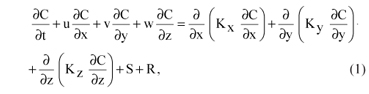
where C is the mean contaminant concentration, S represents the source term, R is the removal term, and u, v, w are the wind components and K_x, K_y and K_z are the eddy diffusivity coefficients along the x, y and z directions, respectively.

Equation 1 was simplified by considering the following assumptions;

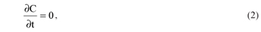
1-Steady-state conditions, that is

2-

3-The mean wind blowing along the x axis, so that v = w = 0,

4-The x transport by the mean flow is greatly outweighs the eddy flux in that direction, that is

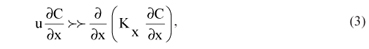
5-There in no source and removal of contaminants , i.e., S = 0 and R = 0.

Under these assumptions Equation 1 reduces to

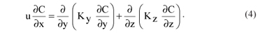
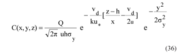
By assuming the Gaussian concentration distribution in crosswind direction (Huang, 1979; Irwin et al., 2007), the solution of Equation 4 in a three dimensional can be written as:

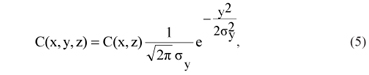
where, C(x,z) is the crosswind integrated concentration and σ_y is the lateral dispersion parameter.

The crosswind integration of Equation 4 from -∞ to + ∞ leads to:

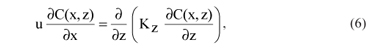
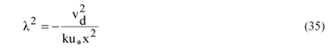
where

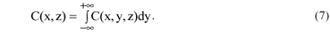
The mathematical formulation of C(x,z) is obtained by solving Equation 6 under the following boundary conditions:

(a) The crosswind-integrated concentration decays in the vertical direction:

(b) The law of conservation of the flux of pollutant can be written as:

where h is the height of the mixing layer, Q is the emission rate and δ (.) is the Dirac delta function.

(c) The dry deposition of pollutants on the ground surface is taken into account through the boundary condition:

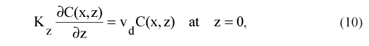
where, v_d is the deposition velocity.

(d) the pollutants are removed immediately upon contact with the top of the mixing layer, i.e.,

The analytic solution of Equation 6 is derived in two cases:

2.1 The first case

The eddy diffusivity depends only on the height z above the ground, and takes the form:

Therefore, Equation 6 becomes:

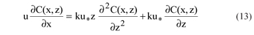
where, k is the von-Karman's constant and is taken to be 0.4, and u_* is the friction velocity.

Using the separation of variables technique:

which transforms Equation 13 into two ordinary differential equations:

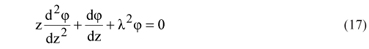
The first equation is:

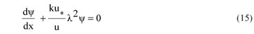
and its solution has the form:

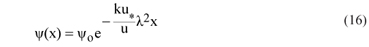
where, -λ² is a separation constant and y_o is an integration constant.

The second equation is:

On using the transformation

The above equation becomes as:

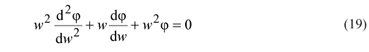
which is the Bessel equation of zero order and its general solution is given by:

where J₀ is the Bessel function of the first kind of order 0, and Y₀ is the Bessel function of the second kind of order 0.

Returning to the original variable, the general solution of Equation 6 can be written as:

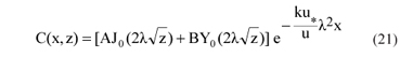
Application of the boundary condition Equation 10 at z = 0 on the above equation, yields B = 0, and Equation 21 becomes as:

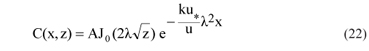
Application of the boundary condition Equation 9 on Equation 22 gives:

Application of the boundary condition Equation 11 on Equation 22 yields:

On putting λ ₌λ_n , (n = 1,2,......), one gets:

So, the values of λ_n can be determined from the zeroes of Equation 24b.

The general solution of Equation 4 takes the form:

2.2 The second case

The eddy diffusivity depends only on the downwind distance x, and has the form:

So, Equation 6 becomes:

The separation of variables technique Equation 14 transforms Equation 27 into two ordinary differential equations;

The first equation is:

and its solution has the form:

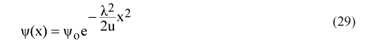
The second equation is:

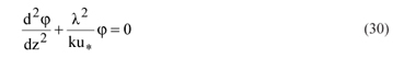
And its solution has the form:

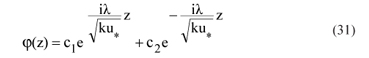
So, the general solution of Equation 6 has the form:

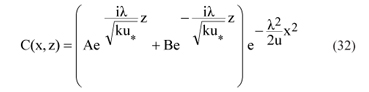
Application of the boundary condition Equation 8 on Equation 32 yields A = 0, and the condition Equation 9 gives:

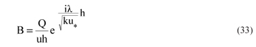
Therefore, Equation 32 becomes as:

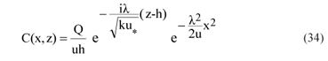
And from the boundary condition Equation 10 we get:

The general solution of Equation 4 can be written as:

3. RADIOACTIVE DECAY

In the case of short-lived radionuclides, the radioactive decay will reduce the concentrations of a radionuclide as it disperses downwind; the corrected concentration can be obtained by multiplying the initial source strength, Q, by the following depletion factor (IAEA, 1982):

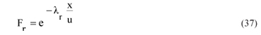
where, λ_r is the radioactive decay constant of the radionuclide with the units of reciprocal time, and represents the fraction of the radionuclides that decay per unit time.

4. STATISTICAL ANALYSIS OF THE MEASURED AND PREDICTED CONCENTRATIONS

The most commonly statistical measures used for model evaluation were chosen for the present analysis are (Fariba and Hanadi, 2004 and Davidson et al., 2005):

(1) The normalized mean square error is defined as

where C_o and C_p are the observed and predicted concentrations, respectively. It gives information on the overall deviations between the predicted and observed concentrations. A good model should have NMSE value close to zero

(2) The correlation coefficient

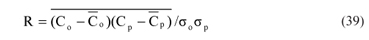
where σ_o and σ_p are the standard deviations of the observed and predicted concentrations, respectively. The value of R lies between 0 and 1 and for good performance of a model it should be close to unity.

(2) The fractional bias is given by

It provides information on the tendency of the model to overestimate or underestimate the observed concentrations. A good model should have FB value close to zero.

(4) Factor of two and factor of five:

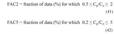
The value of FAC2 and FAC5 should be close to unity for good model performance.

5. AN APPLICATION ON A RESEARCH REACTOR

The resulting analytical models are used to calculate the concentration of Iodine I-131 released from the Research Reactor. The data used was obtained from the experiments performed to collect air samples around the Reactor under neutral and stable conditions. The samples were collected at a height of 0.7 m above the ground. The emissions were released from a stack of height 27 m. The roughness length of the area around the Reactor was 0.6 m (Khaled, 2009). The deposition velocity of Iodine v_d = 0.01 m/s and the decay constant l_r of Iodine I-131 has the value 9.95x10^-7 per second.

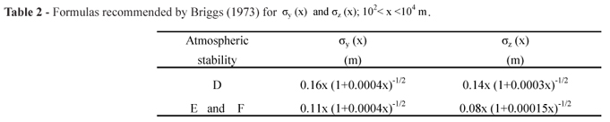
Summary of the meteorological conditions and the observed concentrations during the experiments presented in Tables 1, ³ and ⁴ are taken from Khaled, (2009). The values of lateral dispersion parameter σ_y were calculated using the Briggs (1973) formulae in urban conditions, see Table 2.

6. RESULTS AND DISCUSSIONS

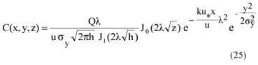
The concentrations of Iodine I-131 below the centerline of the plume C (x, 0, z) in Bq/ m³ were calculated in neutral and stable atmosphere by using the new models Equations 25 and 36, the results are presented in ^{Tables 3} and ⁴. The comparisons between the observed and predicted concentrations of I-131 in neutral and stable conditions are represented graphically as in Figures 1 and 2.

A scatter diagram of the predicted concentrations by the new models and the corresponding observations under stable and neutral cases is shown in Figures 3 and 4, respectively. The dotted lines indicate a factor of two and dashed lines indicate a factor of five departures from a perfect prediction (solid line).

To evaluate the performance of the derived models statistical analysis is performed on the observed and predicted concentrations under stable and neutral conditions. The results of the statistical measures used to evaluate the model performance are shown in Table 5.

^{Tables 3} and ⁴ and Figures 1 and 2 show a very good agreement between the observed and predicted concentrations by Equation 25 under neutral condition, and a reasonable agreement by Equation 36 in stable case. Also, show a less agreement between the observed and predicted values by Equation 25 in stable case and by Equation 36 in neutral case.

Figures 3 and 4 and Table 5 reveal that each of Equation 25 and Equation 36 over predicts the observed concentrations in stable case and under predicts in neutral case.

The statistical measures (Table 5) show that a very good agreement is obtained between concentrations observed and predicted by Equation 25 in neutral conditions, with NMSE and FB values nearest zero, R (0.88), 92% of the predicted concentrations within the factor of two and all the predicted values within the factor of five. Also, show a reasonably agreement by Equation 36 in stable case, with NMSE (0.56) and FB (-0.68), R (0.82), FAC2 (54%), and FAC5 (85%). Each of Equation 25 in stable case and Equation 36 in neutral case gives similar values for the statistical indices which indicate a less agreement between observed and predicted values.

7. SUMMARY AND CONCLUSIONS

An analytical solution of the three dimensional advection-diffusion equations has been formulated in two cases where, the vertical eddy diffusivity is taken to be dependent on: (a) the downwind distance x only and (b) the height z only. The solution is based on the assumption that the concentration distribution of pollutants in the crosswind direction has a Gaussian shape and the wind speed is constant the dry deposition of the diffusing particles on the ground is taken into consideration throughout the boundary conditions. The resulting formulae have been applied to calculate the concentration of I-131 using data collected from the diffusion experiments conducted around a Research Reactor. Statistical analysis was performed on the observed and predicted concentrations to evaluate the performance of the derived models. The results of this study have been discussed and presented in tables and illustrative figures. The statistical measures reveal that Equation 25 presents a very good performance in neutral case.

8. REFERENCES

Received May 2013

Accepted April 2014

• BRIGGS, G. A. Diffusion estimation for small emissions, ATDL Contrib. 79 (draft), Air Resource Atmospheric Turbulence and Diffusion Laboratory, Oak, Ridge, 1973.
• Davidson M. M., Tirabassi T., Vilhena M. T., Carvalho, J. C. A semi-analytical model for the tritium dispersion simulation in the PBL from the Angra I nuclear power plant. Ecological Modelling, v. 189, p. 413-424, 2005
• FARIBA M., HANADI S. R.: Modeling point source plumes at high altitudes using a modified Gaussian model. Atmospheric Environment, v. 38, p. 821-831, 2004.
• HUANG, C. H. A theory of dispersion in turbulent shear flow. Atmospheric Environment, v. 13, p. 453-463, 1979.
• IAEA: Generic models and parameters for assessing the environmental transfer of radionuclides from routine releases. Safety series, n. 57, Vienna, 1982.
• IRWIN, J. S.; PETERSEN, W.B.; HOWARD, S.C. Probabilistic characterization of atmospheric transport and diffusion. Journal of Applied Meteorology, 46, 980-993, 2007.
• KHALED S. M. E.: Gaussian plum model parameters for ground level and elevated sources derived from the atmospheric diffusion equation in the neutral and stable conditions. Arab Journal of Nuclear Sciences and Application, v. 42, n. 3, 2009.
• LIU, M.K., SEINFELD, J.H.: On the validity of grid and trajectory models of urban air pollution. Atmospheric Environment, v. 9, p. 555-574, 1975.
• NIEUWSTADT, F.T.M.: An analytical solution of the time dependent, one-dimensional diffusion equation in the atmospheric boundary layer. Atmospheric Environment, v. 14, p. 1361-1364, 1980.
• PASQUILL,F., AND F. B.SMITH: Atmospheric diffusion John Wiley and Sons, 1983, 437 pp.
• RUNCA, E.: A practical numerical algorithm to compute steady state ground level concentration by a K-model. Atmospheric Environment, v. 16, p. 753-759, 1982.
• RUNCA, E., SARDEI, F.,: Numerical treatment of time dependent advection and diffusion of air pollutants. Atmospheric Environment, v, 9, p. 69-80, 1975.
• SEINFELD J.H.: Atmospheric Chemistry and Physics of Air Pollution, Wiley, New York, Ch13 , pp 564-569, 1986.

Publication Dates

• Publication in this collection
  27 Aug 2014
• Date of issue
  Sept 2014

History

• Received
  May 2013
• Accepted
  Apr 2014