Climate analysis using neural networks as supporting to the agriculture

Análise Climática utilizando redes neurais como apoio à agricultura

Abstracts

Abstract

The aim of this study is to conduct climate forecasting with models of artificial neural networks as a tool in the decision-making process for the planting of some types of agricultural products. A database with the main climate elements was built from the National Institute of Meteorology (INMET), and those elements that influenced the average temperature value the most were found at a significance level of 0.05. Models of Artificial Neural Networks were developed and tested using Mean Absolute Deviation (MAD), Mean Squared Error (MSE), Root-Mean Squared Error (RMSE), and Mean Absolute Percentage Error (MAPE), before being linked to the best agricultural cultivation forecast value. Twelve neural networks were elaborated, eight of them are related to the temperature forecast and the other four are related to the precipitation forecast. The networks that showed the best performance are those that consider all the elements of climate. It is possible to conclude that the artificial neural networks showed an adequate performance in predicting chaotic time series, and that their results were therefore linked to the optimum cultivation to use for each forecast. A schedule is supplied at the end, indicating the ideal time to plant each of the crops evaluated. Carrot is found to be the best suited crop for the forecasted range over the next five years.

Keywords:
Artificial neural networks; Climate forecasting; Apple crops; Grape crops; Carrot crops; Tomato crops; Cultivation schedule

Resumo

O objetivo desse trabalho é fazer a análise climática, utilizando modelos de redes neurais artificiais, como auxílio no processo de tomada de decisão no plantio de alguns tipos de produtos agrícolas. Um banco de dados com os principais elementos do clima foi construído a partir do site do INMET (Instituto Nacional de Meteorologia) e desses elementos foram identificados, em um nível de significância de 0,05, os que mais influenciavam no valor da temperatura média. Modelos de Redes Neurais Artificiais foram criados e avaliados por meio do MAD (Mean Absolute Deviation), MSE (Mean Squared Error), RMSE (Root-Mean Squared Error) e MAPE (Mean Absolute Percentage Error), e finalmente, associou-se o valor da previsão com o melhor cultivo agrícola a ser aplicado. Foram elaboradas 12 redes neurais, oito são referentes à previsão da temperatura e as outras quatro à previsão da precipitação. As redes que demostraram melhor desempenho são as que consideram todos os elementos do clima. É possível concluir que as redes neurais demostraram um desempenho adequado na previsão de séries temporais caóticas, e consequentemente, tiveram o seu resultado associado com o melhor cultivo a ser aplicado para cada previsão. Um cronograma é apresentado no final, sugerindo a melhor época para plantar cada uma das culturas estudadas. Observa-se que para os próximos cinco anos, o cultivo mais adequado à faixa prevista é o da cenoura.

Palavras-chave:
Redes neurais artificiais; Análise climática; Culturas de maçã; uva; tomate de cenoura; Cronograma de plantio

1 Introduction

According to the results of the Institute of Agricultural Economics (IEA) presented in May 2020 (IEA, 2020), the Brazilian foreign trade was not in deficit only due to the agribusiness performance, as other sectors of the economy produced a deficit of US$21.02 billion in the first five months of 2020, with exports of US$42.52 billion and imports of US$63.54 billion. In the period under review, the agribusiness surplus was US$36.59 billion, which represents an increase of 11.0% when compared to the period between January to May 2019. The share of agriculture exports in the national total increased by 6.9%, while the share of imports decreased by 0.6% during the period studied (IEA, 2020).

According to Radin & Matzenauer (2016), climate change and environmental temperature have a direct impact on the agricultural industry, as these elements might interfere with soil, harvesting, irrigation, and even the process of shipping and storing products.

As can be seen, climate change has a significant impact on agriculture, making weather forecasting a key part of the decision-making process. According to Sampaio & Dias (2014), the models of weather forecasting began in the 19th century, when meteorologist Cleveland Abbe used mathematical approximations to obtain a predictive model of the state of the atmosphere.

Artificial Neural Networks (ANN can be compared with statistical techniques of pattern recognition and learning as well as performing time series predictions, which is a widely used method of calculation in AI). In the paper of Dantas et al. (2016), Muntaser et al. (2017) and Norvig & Russell (2013), the Neural networks were used to perform precipitation and stock market forecasts, respectively, with satisfactory results.

This study seeks to do climate forecasting using artificial neural networks to aid in the cultivation of certain crops such as carrots, apples, grapes, and tomatoes, as well as help to the development of agribusiness in the Caxias do Sul region and throughout Brazil. Caxias do Sul is the second largest city in the state of Rio Grande do Sul, and is known for its grape cultivation, wine production, and metalworking industry. According to data on agricultural production in Caxias do Sul in 2016, the four largest productions are the target crops of this study: apples, grapes, tomatoes, and carrots (IBGE, 2017; Caxias do Sul, 2018) .

2 Artificial neural networks for climate forecasting

Plant cycles are related to variations in environmental conditions and characteristics of each plant species. With knowledge of the crop to be cultivated and the climate of the region, it is possible to plan the irrigation system, fertilizers, and harvesting, among other factors, allowing for improved profitability and quality (Fiorin & Ross, 2015).

2.1 Impact of climate factors on carrot, apple, grape, and tomato crops

According to Fiorin & Ross (2015), climatic factors are aspects that interfere with climatic elements. The non-uniform distribution of solar radiation and the temperature of the earth's surface influence agriculture in terms of cultivated plant species. Warm-season crops grow and develop between 25 °C to 30 °C and can be planted all year in the tropical zone, but they must be grown during the warm months in subtropical regions like Rio Grande do Sul (September to March). Grape and apple cultures are included in this group. Cold-season crops thrive in temperatures ranging from 15 °C to 25 °C and can be cultivated in the southern states during the cooler months of April through August.

The minimum temperature range for tomato germination is between 8 °C and 11 °C, while the optimum range is between 16 °C and 29 °C. During cultivation, the average temperature should be 21 °C, resisting temperatures from 12 °C to 34 °C. Temperatures above 28 °C cause the fruits to turn yellow, and temperatures near 32 °C cause flower abortion, poor fruit development, and hollow fruit formation. Temperatures above 26 °C reduce the crop cycle. The ideal temperature range for tomato production is between 20 °C and 24 °C (Silva et al., 2006).

In terms of precipitation, tomatoes are considered as plants that require a lot of water, but excessive rain can harm its cultivation. High rainfall and high relative humidity facilitate the spread of diseases, requiring constant spraying of pesticides. Excessive precipitation can also impact fruit quality. The water requirement of tomato plants ranges from 400 mm to 600 mm (Silva et al., 2006; Neves et al., 2013).

Cold temperature is an important element in the apple growing process. This culture must be exposed to a temperature below 7.2 °C for 800 hours in a standard and universal manner. However, during the vegetative stage the ideal temperature range for its development is between 18 °C and 23 °C, with a maximum temperature of 25 °C. Temperatures below 10 °C should be avoided during flowering, as this makes fruit fixation and growth difficult, and because exceptionally low temperatures impair pollination insect activity. Extremely high temperatures above 30 °C can cause bark burns (Braga et al., 2001; Fioravanço & Santos, 2013).

Rain is another significant factor in apple agriculture, particularly during the fruit growth period. Water constraints might cause the fruit to shrink in size and nutrition absorption to suffer. Apple trees require a minimum of 700 mm and a maximum of 1,700 mm of rain per year. Plant development is also influenced by precipitation distributions; persistent rains during flowering reduce production, and excessive amounts of rain in a short period of time can suffocate roots, impairing nutrient absorption (Fioravanço & Santos, 2013).

Several aspects of grape agriculture are influenced by the weather, including cycle duration, fruit quality, plant health, and vine productivity. It is a temperate climate culture that requires between 50 and 400 hours of temperatures below 7 °C (Leão et al., 2009).

Plant photosynthetic activity is influenced by air temperature because it requires biological reactions involving temperature-dependent catalysts. These reactions are slower at temperatures below 20 °C, intensifying with increasing temperature until reaching a maximum value in the range of 25 °C to 30 °C. The ideal average temperature for vine planting lies between the ranges of 15 °C to 30 °C (Teixeira et al., 2002).

During the rest period, the vine can withstand negative temperatures between the range of -10 °C to -20 °C, but vegetation starts to grow with temperatures above 10 °C. During the vegetative period, plants can adapt to temperatures of up to 35 °C. In terms of precipitation, the months of November and April have a historical average of 570 mm, though this can vary up to 680 mm. (Nachtigal & Mazzarolo, 2008; Leão et al., 2009).

Carrot is a tuberous root vegetable grown primarily in the Southeast and South regions of Brazil. It has a lot of vitamin A, soft texture, and a pleasant flavour, and it may be eaten raw. It is also used as raw material by food processing industries (Souza et al., 1999). Temperature is a relevant variable in root production. Temperatures between 10 °C and 15 °C promote elongation and the formation of the unique colour; however, temperatures above 21 °C inhibit root and colour development. Temperatures exceeding 30 °C shorten the vegetative cycle of the plant, reducing its productivity. Another aspect that has a detrimental impact on it is excessive air humidity during hot weather, which encourages the development of plant diseases. During the germination period, the ideal temperature range is between 20 °C to 30 °C (Vieira & Pessoa, 2008).

The productivity and quality of carrot roots are both affected by soil moisture. The water requirement for carrots is in the range of 350 mm to 500 mm. This crop is sensitive to water deficit. Excess water encourages the spread of diseases and obstructs the soil's ability to absorb oxygen, water, and nutrients (Marouelli et al., 2007; Souza et al., 1999).

Temperature and unit, as well as other climatic factors, have a significant influence on the four crops. The Materials and Methods section explains how climate forecasting is performed and how advantageous planting times are identified using these forecasts.

2.2 Artificial neural networks as a forecasting model

Artificial Neural Networks (ANNs) are based on the functioning of the neurons of the human brain that are responsible for information processing. ANNs can be characterized as computational models that have adaptation, learning, pattern recognition and data organization skills, whose mechanism is based on parallel processing (Rabuñal & Dorado, 2006; Krose & Smagt, 1996). Since their introduction, they have primarily been used to anticipate weather, energy consumption and demand, as well as exchange rates and stock prices (Wang et al., 2012; Abhishek et al., 2012; Liao & Wang, 2010).

The significance of the study is to link artificial neural networks as a method, climate characteristics as a sine qua non condition, and the best time to plant crops as conclusion. In this context, there are few publications relating climate forecasting with agriculture, as well as the application of Artificial Intelligence (AI) tools to solve this type of problem. The current study focuses on local application, considering the unique climate characteristics of the region.

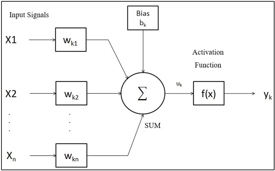
The basic processing unit of an ANN is the artificial neuron which has the capacity to store experimental knowledge. Figure 1 shows the structure of an artificial neuron. In a network, these neurons are distributed in certain architectures to perform data processing. Since the desired answer for that data set is also provided within the input data of a network, the process of learning a network is conducted by adjusting the synaptic weights. As a result, the network compares the number it generated with the desired value, thus generating an error signal that is sent back and adjusted to the synaptic weights to minimize the error (Kopiler et al., 2019).

Figure 1
Structure of an artificial neuron.

In Figure 1 each input signal has a weight. The synaptic weight w_kj is multiplied by a signal x_jat the input of a neuron, where the index k refers to the neuron where the information input occurs, and the j refers to the input terminal. Synaptic weights can have positive or negative values, and their purpose is to weight the value of each input. As a result, the adder sums the input signals after multiplying them by their corresponding weights. The activation function is responsible for limiting the output amplitude of a neuron. The term bias (b_k) is applied externally, and its function is to increase or decrease the input of the activation function, which can be a negative or positive value. An artificial neuron can be mathematically written according to Equations 1 and 2 (Haykin, 2001).

$$u_k={\displaystyle \sum _{j=1}^m{w}_{kj}{x}_j}$$ (1)

$$y_k=\phi \left(u_k+b_k\right)$$ (2)

In the equations, the values of x₁, x₂, ..., x_n represent the input signals; w_k1, w_k2, ..., w_kn refer to the synaptic weights of neuron k, while u_k is the sum function. In the second equation, b_k represents the bias, $\phi$ represents the activation function and y_k is the output signal of the neuron.

According to Liu et al. (2016), the activation function ($\phi )$aggregates all input values, transforming this data into new numbers). It is normally a non-decreasing function of the total input of the unit. There are numerous types of activation functions. Some examples are linear functions, tangent hyperbolic function, Gaussian function, radial basis function, etc.

The application of ANNs is present in several areas, as it can learn and adapt to the environment in which it operates. It is an efficient method for calculations that require large amounts of data. In certain cases, such as in nuclear physics, the calculation to describe the state of a particular atom or particle contains a lot of information, to the point where numerical and probabilistic models only give limited responses, and it is possible to get a more precise result by using ANNs. In the research by Carleo & Troyer (2017), the authors use this technique to calculate the value of the wave function, obtaining relatively accurate results. Pattern and picture recognition is another application for ANNs, as demonstrated the research by Fei et al. (2017), who developed two models for predicting venous thrombosis in patients diagnosed with acute pancreatitis. ANNs had an accuracy of 83.3% in this study, while logistic regression, another prediction technique, had an accuracy of around 60%.

3 Material and methods

The study is of a retrospective type, based on secondary historical data. The database was built using the National Institute of Meteorology (INMET) website, which was used to download monthly average temperatures of the city of Caxias do Sul from January 31, 1961, to December 31, 2017. A 56-year history was obtained with the variables that were available. Data were obtained with a monthly step. An electronic spreadsheet was used to calculate the quarterly average of all variables for improved organization. The period between 1985 and 1991 was excluded from the analysis, because the station did not record the measurement of several variables in this interval. Therefore, the bank includes 200 values for each of the variables studied. When INMET did not store a single isolated variable in each period, the value of that variable was assigned as the average of the previous and succeeding periods.

After creating the database, an analysis of variance (ANOVA) was used to see if there was a difference in the average temperature in connection to the seasons that was significant at the 0.05 level (Hair et al., 2005; Fávero et al., 2009). This was confirmed, and four predictions, one for each season of the year, were made. The characteristic effects caused by meteorological changes, such as El Niño and La Niña, which induce fluctuations in rainfall and temperature in the southern region of Brazil (Jacóbsen et al., 2004),are intrinsic in the data analysed. Such atypical periods were not analysed separately and can be considered a limitation of the study. In the analysis, the values of peaks and valleys were not disregarded. The climate forecast is made using Artificial Neural Networks, a statistical methodology based on Artificial Intelligence (AI).

3.1 Elaboration of the artificial neural network model for prediction

The AI model used in this study is based on the concept of Artificial Neural Networks. By premise, these models consider input values, which are called “target”. Based on these values, the mathematical network model aims to adapt to these values, not simply memorize them, but also recognize their behaviour over time. The target data for this study are the quarterly average temperature (divided by seasons) of the database created, as well as the variables that reflect climate factors (Figure 2). With these input data, the mathematical prediction model is calibrated with optimization algorithms, aiming to minimize the error obtained by the network.

Figure 2
Network architecture used in the study.

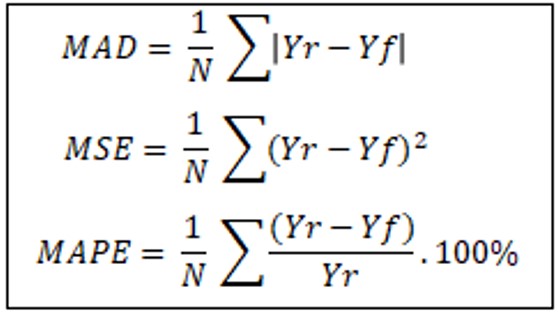
The ANN used is a time-delayed Multilayer Perceptron (MLP) with a fed-forward layer of hidden neurons trained by means of the backpropagation algorithm (Haykin, 2001; Krose & Smagt, 1996). The last five periods were removed from the training portion and used for testing and calculating the performance of the network. The network's performance is assessed by the Mean Absolute Percentage Error (MAPE), with a result of less than 10% for temperature forecasts and less than 30% for precipitation forecasts indicating that the network is appropriate. Other performance indicators are also calculated for comparison: Mean Absolute Error (MAD), Mean Squared Error (MSE) and Root-Mean Squared Error (RMSE). Figure 3 shows how these indicators are calculated. The RMSE value is calculated from the square root of the MSE value. In all instances, the lower the indicator value, the better the network performance.

Figure 3
Performance indicators used in the study.

Yr = actual value measured by the station

Yf = value predicted by the network

N = number of periods analysed

Table 1 shows the variables (X1 to X9) that tend to influence the dependent variable (Y), which is called average temperature.

Table 1
Identification of variables that influence the average temperature.

Variables	Units
Average temperature (Y)	°C
Minimum average temperature (X1)	°C
Average maximum temperature (X2)	°C
Tar evaporation (X3)	mm
Number of days with precipitation (X4)	Quantity
Relative humidity (X5)	%
Average wind speed (X6)	mps
Cloud cover average (X7)	Tenths
Average maximum wind speed (X8)	mps
Total precipitation (X9)	mm

The Artificial Neural Network was created with the help of the Python software. Two vectors were informed for the ANN software supplement, one containing the targets and the other containing the independent variables. Subsequently, the network was trained by backpropagation, generating forecasts for future periods. From the identified elements that most influence the climate, three networks were developed (Table 2), the first to predict future quarterly average temperature, the second to predict future quarterly average precipitation, and the third to predict future monthly average temperature.

Table 2
ANNs created.

Network number	Input data	Output
1	All climate elements	Future precipitation
2	Significant elements of the climate	Future temperature
3	All elements of the climate	Future temperature

3.2 Identification of the ideal features for the cultivation of the four types of crops

Table 3 was created using the bibliographical review and shows the ideal rainfall data, temperature range, and crop growth period for each type of crop. The value predicted by the network is compared with this temperature and precipitation range.

Table 3
Cultivation relationship with temperature and precipitation.

Cultivation	Precipitation	Temperature range (°C)	Development time (years)
Tomato	400-600 mm	20 to 24	0.5
Apple	700-1700 mm	18 to 23	1.5
Grape	570-680 mm	15 to 30	1
Carrot	350-500 mm	15 to 21	0.5

3.3 Most significant elements for the average temperature

A multiple linear regression was used to determine which of the nine variables (Table 1) are statistically significant at the 0.05 level in connection to the average temperature, the dependant variable. Because there are significant changes in temperature within each season in the city of Caxias do Sul, a linear regression was conducted for each season of the year. The analysis was performed with a 95% confidence level in the SPSS® statistical software. The average temperature (Y) has a high explained variance in all four seasons of the year (Table 4), and the variable X1, minimum average temperature (Table 1), is present in all models of each season and has the greatest influence on the average temperature in the spring, summer, and autumn. The variable X2, average maximum temperature, exerts greater influence on the average temperature model only in the winter season.

Table 4
Multiple linear regression for the four seasons of the year.

Season	R2	Significant variables	Largest linear coefficient value in the equation
Summer	0.969	X1, X2 and X3	X1
Autumn	0.930	X1	X1
Winter	0.964	X1, X2, X6 and X8	X2
Spring	0.975	X1, X2, X6 and X8	X1

• Dependent variable: Y = average temperature. N = 200.

4 Results presentation

The networks used had 10 hidden neurons and a two-period delay. Regarding the sample data, 90% of the data was used for training and 10% for testing and validation.

We developed a network for each season, as the Analysis of Variance (ANOVA) revealed that there is a substantial difference in the average temperature as a function of the season of the year. We developed a total of 12 ANNs, eight of which are connected to forecasting the average temperature, with the first four networks taking into consideration all climatic parameters as input, and the remaining four networks only considering elements with a significance level of 0.05. (Table 4). Finally, the last four networks perform the precipitation forecast from all elements of the climate.

4.1 Climate forecasting with the use of ANNs

Table 5 presents the results of temperature prediction, four of which use all independent variables, while the others consider only the variables identified as significant. Table 5 shows that the networks that performed best in spring, summer and winter were those that used all parameters of the created database, as the values of all indicators are smaller for them. As regarding autumn, the network that performed the best was the one that only included the significant factors. Therefore, for the phase of association of the predicted temperature with the cultivation the networks that consider all parameters for summer, winter and spring are used, while the association of cultivation for autumn uses the net that uses only the significant parameters.

Table 5
ANNs comparison of performance indicators developed for temperature.

ANN	MAD	MSE	RMSE	MAPE
Summer all parameters	0.7	0.9	0.95	3.42%
Summer significant parameters	0.79	1.06	1.03	3.84%
Winter all parameters	1.27	2.10	1.44	8.44%
Winter significant parameters	2.00	4.35	2.09	13.56%
Autumn all parameters	1.02	1.12	1.06	6.85%
Autumn significant parameters	0.59	0.49	0.70	4.02%
Spring all parameters	0.55	0.53	0.73	2.96%
Spring significant parameters	1.24	1.81	1.35	6.67%

• N= 200. Dependent variable (Y) = average temperature.

Figure 4 illustrates the four artificial neural networks used to predict temperature. The red line represents the actual values extracted from the INMET database for the period considered in the survey. The blue line represents the best temperature forecast obtained for each season of the year.

Figure 4
ANNs for temperature prediction.

4.2 Precipitation prediction using ANNs

The precipitation forecast was performed by providing the same variables used in temperature forecasting, but in this case, the dependent variable (Y) is total precipitation, and the others are independent variables, including average temperature. The forecasts were divided into four, where each network predicts the precipitation of one season of the year. Observing Table 6, it is possible to observe that the forecasts that presented the lowest error values were those in the spring and autumn. In comparison with temperature forecasts, the precipitation networks, in general, present higher error values.

Table 6
Comparison of ANNs performance indicators developed for precipitation.

ANN	MAD	MSE	RMSE	MAPE
Summer precipitation	55.14	4641.15	68.13	29.62%
Winter precipitation	32.41	1328.36	36.45	21.46%
Spring precipitation	34.91	2198.2	46.88	16.39%
Autumn precipitation	27.86	1126.52	33.56	17.19%

• N = 200. Dependent variable (Y) = precipitation.

Figure 5 illustrates the four artificial neural networks used to forecast precipitation. The red line represents the actual values extracted from the INMET database for the period considered in the survey. The blue line represents the precipitation forecast obtained for each season of the year.

Figure 5
ANNs for precipitation prediction.

4.3 Analysis of forecast association with cultivation

The result of the prediction of temperature and precipitation is associated with the ideal cultivation. Table 6 is used as a parameter to make the comparison between the ideal ranges for each crop and the predicted values. Table 7 presents the predicted temperature values (°C), while the precipitation forecast (mm) for future periods is presented in Table 8.

Table 7
Temperature forecast for future periods.

Year	Summer	Winter	Autumn	Spring
2018	21.60	13.29	15.14	18.55
2019	21.76	15.86	15.54	18.63
2020	21.58	14.69	15.18	18.27
2021	21.48	15.68	15.72	18.30
2022	21.53	15.31	14.96	18.38

Table 8
Precipitation forecast for future periods.

Year	Summer	Winter	Autumn	Spring
2018	111.61	175.04	127.66	183.41
2019	222.13	124.63	269.01	219.91
2020	164.13	257.33	148.07	173.71
2021	128.40	249.18	242.03	182.11
2022	146.23	266.09	168.48	169.14

• N = 200.

The selection of the best crop was carried out considering the period of development of each plant: one year for grapes, one and a half years for apples and six months for carrots and tomatoes. Therefore, the average temperature and the sum of precipitation were used for their respective periods.

Figure 6 presents the schedule created exclusively on the values of temperature and precipitation estimates for the Caxias do Sul location. and in the ideal ranges of each crop. In some cases, the predicted value was approximated by the value of one of the ideal ranges. The painted spaces indicate when that crop should be planted within that period. Carrots appear to be the crop that best fits the forecast ranges, being planted in most periods.

Figure 6
Suggested Cultivation Schedule based on temperature and precipitation forecasts.

The years 2018 and 2020 presented the ideal characteristics for growing grapes, while apples should ideally be planted at the end of 2021. The tomato was the only crop where forecast conditions did not meet their ideal range; however, the forecast value could be approximated in the first six months of 2019.

5 Discussion and final considerations

In this study, the artificial neural network model demonstrated its ability to enable decision-making on the ideal time to plant apple, grape, tomato, and carrot crops, precisely based on climate variables in the city of Caxias do Sul, based solely on temperature and precipitation forecasts. These forecasts, along with other important criteria for the cultivation, lead farmers to make more assertive decisions, offering a broader range of analysis on the risk variables for each cultivation and loss control. Climate analysis, based on temperature and precipitation forecasts, is another aspect that, when combined with other elements such as topography, soil conditions, and unexpected weather effects, tends to improve farmer or agriculture sector decision-making.

The originality of this study is associated with the triad of climate analysis as the objective, artificial neural networks as forecasting method, and the recommendation of an annual timetable for cultivation in each place as the major result. In our research, we created models to forecast the average temperature and precipitation for the city of Caxias do Sul. During the study, we were able to identify that there is a difference with significance at the level of 0.05 in the average temperature and precipitation due to the season of the year, therefore we created forecast models for each one of the seasons separately.

Because the empirical behaviour of temperature as a function of time is chaotic, the prediction model chosen was based on an artificial intelligence technique known as Artificial Neural Networks. This technique is distinguished by its ability to learn from examples and adapt to the environment in which it is embedded, making it ideal for predicting non-linear series.

The analysed data were obtained from the INMET website. Following the initial treatment of this data, we divided it by season of the year, and a multiple linear regression was developed for each season, identifying the major factors that influenced the average temperature. The result of the regression for all cases was satisfactory. The generated model was significant with an R² value greater than 0.9. Variables significant at the 0.05 level were used as input data in the ANN model created.

We also used a multiple linear regression to develop a prediction model, to compare the obtained value with the ANN value. The regression model created was advanced in time, adapting to the temperature value of a certain period using inputs from five previous periods. However, the generated model presented an unsatisfactory R² value, making it impossible to carry out a forecast by this method.

We developed a total of 12 ANNs, eight representing the networks referring to temperature forecasts and the other four referring to precipitation forecasts. In general, the ANNs showed an adequate performance in both cases. The networks chosen for comparison with the crop ranges were those that considered all elements of the climate, except for the autumn network. This one considers only the significant elements of the climate. The networks selected for comparison had the lowest error values which were calculated with the proposed performance indicators.

Precipitation networks showed a relatively greater error than temperature networks. Therefore, we suggest a more detailed study of the precipitation variable through a non-linear regression analysis or using other elements for the network definition.

The ideal ranges of temperature and precipitation for each crop studied were created from the literature review on the subject, specially from articles and books on the subject. We compared the result of the best network for each season with the value of the ideal ranges, thus associating the respective period with cultivation. Thus, the aim of the study was met, and it was concluded with the creation of a cultivation schedule based on the results of the networks and the identified ideal ranges. It is possible to highlight that carrot cultivation is the most appropriate for the entire period studied.

6 Limitations of the study and suggestions for future research

As a limitation of the study, there is the fact that some periods do not have their variables measured by the meteorological station.

The use of only one network typology with the same training and testing parameters, as well as the same number of hidden neurons, should be considered a limitation.

Factors such as soil, topography and others were not considered in the network input data. Only variables related to the climate of the studied region, the city of Caxias do Sul, were considered, but this does not rule out the possibility of associating other factors with the forecast in future research. This new approach will allow comparisons to be made and should contribute to the refinement of the forecasting model.

Another meteorological aspect is the El Niño and La Niña effects on climate variation, which were present in some periods of the analysed data. These effects affect temperature, precipitation, and other variables that are also presented in the INMET database. The results of these effects are thought to be already included in the consolidated measures of the variables, which are not highlighted in the database because they are classified as atypical natural effects. The data corresponding to the atypical periods of the studied variables was not stratified to be analysed separately, as there is no mention in the database of the occurrence of these effects. Temperature, average temperature, and precipitation data were all treated at their absolute values, as shown in the database (INMET, 2018b). Future research could stratify and verify whether there is a significant difference in the propositional model for cultivation when El Niño and La Niña are present versus when they are not.

• Financial support: None.
• How to cite: Borella, L. C., Borella, M. R. C., & Corso, L. L. (2022). Climate analysis using neural networks as supporting to the agriculture. Gestão & Produção, 29, e06. http://doi.org/10.1590/1806-9649-2022v29e06

References

• Abhishek, K., Singh, M. P., Ghosh, S., & Anand, A. (2012). Weather forecasting model using Artificial Neural Network. Procedia Technology, 4, 311-318. http://dx.doi.org/10.1016/j.protcy.2012.05.047
  » http://dx.doi.org/10.1016/j.protcy.2012.05.047
• Braga, H. J., Silva, V. P., Pandolfo, C., & Pereira, E. S. (2001). Zoneamento de riscos climáticos da cultura da maçã no estado de Santa Catarina. Revista Brasileira de Agrometeorologia, 9(3), 439-445. Retrieved in 2018, October 4, from http://www.cnpt.embrapa.br/pesquisa/agromet/pdf/revista/cap7.pdf
  » http://www.cnpt.embrapa.br/pesquisa/agromet/pdf/revista/cap7.pdf
• Carleo, G., & Troyer, M. (2017). Solving the quantum many-body problem with artificial neural networks. Science, 355(6325), 602-606. http://dx.doi.org/10.1126/science.aag2302 PMid:28183973.
  » http://dx.doi.org/10.1126/science.aag2302
• Caxias do Sul. Prefeitura. (2018). Apresentação. Retrieved in 2018, September 3, from https://caxias.rs.gov.br/cidade
  » https://caxias.rs.gov.br/cidade
• Dantas, D., Luz, T. M. O., Souza, M. J. H., Barbosa, G. P., & Cunha, E. G. S. (2016). Uso de Redes Neurais Artificiais na previsão da precipitação de períodos chuvosos. Revista Espinhaço, 5(1), 10-17. Retrieved in 2018, August 22, from http://revistaespinhaco.com/index.php/journal/article/view/96/90
  » http://revistaespinhaco.com/index.php/journal/article/view/96/90
• Fávero, L. P., Belfiore, P., Silva, F. L., & Chan, B. L. (2009). Análise de dados: modelagem multivariada para tomada de decisões (2ª ed.). Rio de Janeiro: Elsevier.
• Fei, Y., Hu, J., Li, W. Q., Wang, W., & Zong, G. Q. (2017). Artificial neural networks predict the incidence of portosplenomesenteric venous thrombosis in patients with acute pancreatitis. Journal of Thrombosis and Haemostasis, 15(3), 439-445. http://dx.doi.org/10.1111/jth.13588 PMid:27960048.
  » http://dx.doi.org/10.1111/jth.13588
• Fioravanço, J. C., & Santos, R. S. S. (2013). Maçã: o produtor pergunta, a Embrapa responde. Brasília: Embrapa. Retrieved in 2018, October 4, from https://ainfo.cnptia.embrapa.br/digital/bitstream/item/122887/1/Maca-o-produtor-pergunta-a-Embrapa-responde.pdf
  » https://ainfo.cnptia.embrapa.br/digital/bitstream/item/122887/1/Maca-o-produtor-pergunta-a-Embrapa-responde.pdf
• Fiorin, T. T., & Ross, M. (2015). Climatologia agrícola. Santa Maria: Rede E-tec Brasil. Retrieved in 2018, September 25, from http://estudio01.proj.ufsm.br/cadernos_fruticultura/terceira_etapa/arte_climatologia_agricola.pdf
  » http://estudio01.proj.ufsm.br/cadernos_fruticultura/terceira_etapa/arte_climatologia_agricola.pdf
• Hair, J. F., Black, W. C., Babin, B. J., Anderson, R. E., & Tatham, R. L. (2005). Análise multivariada de dados (5ª ed.). Porto Alegre: The Bookman.
• Haykin, S. (2001). Redes neurais princípios e prática (2ª ed.). Porto Alegre: The Bookman.
• Instituto Brasileiro de Geografia e Estatística – IBGE. (2017). Caxias do Sul. Retrieved in 2018, September 4, from https://cidades.ibge.gov.br/brasil/rs/caxias-do-sul/panorama
  » https://cidades.ibge.gov.br/brasil/rs/caxias-do-sul/panorama
• Instituto de Economia Agrícola – IEA. Secretaria de Agricultura e Abastecimento. (2020). Balança comercial dos agronegócios paulista e brasileiro, janeiro a maio de 2020. Retrieved in 2020, July 17, from http://www.iea.sp.gov.br/out/TerTexto.php?codTexto=14812
  » http://www.iea.sp.gov.br/out/TerTexto.php?codTexto=14812
• Instituto Nacional de Meteorologia – INMET. (2018b). Sobre o INMET. Retrieved in 2018, October 25, from http://www.inmet.gov.br/portal/index.php?r=home/page&page=sobre_inmet
  » http://www.inmet.gov.br/portal/index.php?r=home/page&page=sobre_inmet
• Jacóbsen, L. O., Fontana, D. C., & Shimabukuro, Y. E. (2004). Efeitos associados a El Niño e La Niña na vegetação do Estado do Rio Grande do Sul observados através do NDVI/NOAA. Revista Brasileira de Meteorologia, 19(2), 129-140.
• Kopiler, A. A., Silva, V. N. A. L., Oliveira, L. A. A., Linden, R., Silva, L. R. A. A., & Fonseca, B. L. C. (2019). Redes Neurais Artificiais e suas aplicações no setor elétrico. Revista de Engenharias da Faculdade Salesiana, 1(9), 27-33.
• Krose, B., & Smagt, P. D. (1996). An introduction to neural networks Amsterdam: The University of Amsterdam.
• Leão, P. C. S., Silva, D. J., & Bassoi, L. H. (2009). Uva. In: J. A. S. Serejo, J. L. L. Dantas, C. V. Sampaio & Y. S. Coelho (Eds.),Fruticultura tropical (Chap 22, pp. 477-509). Brasília: Embrapa.
• Liao, Z., & Wang, J. (2010). Forecasting model of global stock index by stochastic time effective neural network. Expert Systems with Applications, 37(1), 834-884. http://dx.doi.org/10.1016/j.eswa.2009.05.086
  » http://dx.doi.org/10.1016/j.eswa.2009.05.086
• Liu, P., Zeng, Z., & Wang, J. (2016). Multistability of recurrent neural networks with nonmonotonic activation functions and mixed time delays. IEEE Transactions on Systems, Man, and Cybernetics. Systems, 46(4), 512-523. http://dx.doi.org/10.1109/TSMC.2015.2461191
  » http://dx.doi.org/10.1109/TSMC.2015.2461191
• Marouelli, W. A., Oliveira, R. A., & Silva, W. L. C. (2007). Irrigação da cultura da cenoura. Circular Técnica, 48, 1-14. Retrieved in 2018, November 10, from https://ainfo.cnptia.embrapa.br/digital/bitstream/CNPH/33070/1/ct_48.pdf
  » https://ainfo.cnptia.embrapa.br/digital/bitstream/CNPH/33070/1/ct_48.pdf
• Muntaser, J. G. S., Silva, V. P., & Penedo, A. S. T. (2017). Aplicação de redes neurais na previsão das ações do setor de petróleo e gás da Bm & FBovespa. Revista FSA, 14(6), 49-71. http://dx.doi.org/10.12819/2017.14.6.3
  » http://dx.doi.org/10.12819/2017.14.6.3
• Nachtigal, J. C., & Mazzarolo, A. (2008). Uva: o produtor pergunta, a Embrapa responde Brasília: Embrapa. Retrieved in 2018, October 4, from https://www.embrapa.br/busca-de-publicacoes/-/publicacao/125503/uva-o-produtor-pergunta-a-embrapa-responde
  » https://www.embrapa.br/busca-de-publicacoes/-/publicacao/125503/uva-o-produtor-pergunta-a-embrapa-responde
• Neves, S. M. A. S., Seabra, S., Araújo, K. L., Neto, E. R. S., Neves, R. J., Dallacort, R. & Kreitlow, J. P. (2013). Análise climática aplicada à cultura do tomate na região Sudoeste de Mato Grosso: subsídios ao desenvolvimento da agricultura familiar regional.Ateliê Geográfico, 7(2), 97-115. https://doi.org/10.5216/ag.v7i2.23866
  » https://doi.org/10.5216/ag.v7i2.23866
• Norvig, P., & Russell, S. (2013). Inteligência artificial (3ª ed.). Rio de Janeiro: Elsevier.
• Rabuñal, J. R., & Dorado, J. (2006). Artificial neural networks in real-life applications.Hershey: Idea Group Publishing.
• Radin, B., & Matzenauer, R. (2016). Uso das informações meteorológicas na agricultura do Rio Grande do Sul. Revista da Sociedade Brasileira de Agrometeorologia, 24(1), 41-54. http://dx.doi.org/10.31062/agrom.v24i1.24880
  » http://dx.doi.org/10.31062/agrom.v24i1.24880
• Sampaio, G., & Dias, P. L. S. (2014). Evolução dos modelos climáticos e de previsão de tempo e clima. Revista USP, 103(103), 41-54. http://dx.doi.org/10.11606/issn.2316-9036.v0i103p41-54
  » http://dx.doi.org/10.11606/issn.2316-9036.v0i103p41-54
• Silva, J. B. C., Giordano, L. B., Furumoto, O., Boiteux, L. S., França, F. H., Boas, G. L. V., Branco, M. C., Medeiros, M. A., Marouelli, W., Silva, W. L. C., Lopes, C. A., Ávila, A. C., Nascimento, W. M., & Pereira, W. (2006). Cultivo de tomate para industrialização. Retrieved in 2010, November 8, from https://sistemasdeproducao.cnptia.embrapa.br/FontesHTML/Tomate/TomateIndustrial_2ed/clima.htm
  » https://sistemasdeproducao.cnptia.embrapa.br/FontesHTML/Tomate/TomateIndustrial_2ed/clima.htm
• Souza, A. F., Lopes, C. A., França, F. H., Reifschneider, F. J. B., Pessoa, H. B. S. V., Viera, J. V., Charchar, J. M., Mesquita, M. V., Fo., Makishima, N., Fontes, R. R., Marouelli, W. A., & Pereira, W. (1999). A cultura da cenoura. Brasília: Embrapa. Retrieved in 2010, November 10, from https://ainfo.cnptia.embrapa.br/digital/bitstream/item/162021/1/A-cultura-da-cenoura.pdf
  » https://ainfo.cnptia.embrapa.br/digital/bitstream/item/162021/1/A-cultura-da-cenoura.pdf
• Teixeira, A. H. C., Souza, R. A., Ribeiro, P. H. B., Reis, V. C. S., & Santos, M. G. L. (2002). Aptidão agroclimática da cultura da videira no Estado da Bahia, Brasil da videira no Estado da Bahia, Brasil da videira no Estado da Bahia, Brasil. Revista Brasileira de Engenharia Agrícola e Ambiental, 6(1), 107-111. http://dx.doi.org/10.1590/S1415-43662002000100019
  » http://dx.doi.org/10.1590/S1415-43662002000100019
• Vieira, J. V., & Pessoa, H. B. S. V. (2008). Cenoura (Daucus carota). Retrieved in 2010, November 10, from https://sistemasdeproducao.cnptia.embrapa.br/FontesHTML/Cenoura/Cenoura_Daucus_Carota/clima.html
  » https://sistemasdeproducao.cnptia.embrapa.br/FontesHTML/Cenoura/Cenoura_Daucus_Carota/clima.html
• Wang, F., Mi, Z., Su, S., & Zhao, H. (2012). Short-term solar irradiance forecasting model based artificial neural network using statistical feature parameters. Energies, 5(5), 1355-1370. http://dx.doi.org/10.3390/en5051355
  » http://dx.doi.org/10.3390/en5051355

Publication Dates

• Publication in this collection
  07 Mar 2022
• Date of issue
  2022

History

• Received
  11 Feb 2021
• Accepted
  17 Nov 2021