Numerical Results on the Residual Error Indicator for a Contaminant Transport Model

ABSTRACT

In this article, residual indicators were used to characterize the quality of the numerical solution of the advection-diffusion-reaction equation in a saturated porous medium. Both large and small advection regimes were considered. The small advection was exemplified by a problem with constant data, while non-constant data was considered for the large advection regime. In this case, residual quantities associated with the data must be incorporated into the residual estimates related to the spatial approximation and an auxiliary problem must be solved for the correct obtainment of the temporal estimates. The presentation of the residual indicators as a surface on the finite element mesh provides a detailed view of the regions that need refinement, allows to infer the effect of each estimate on the composition of the global estimator and, in addition, allows to follow the evolution of the residual surfaces as the contaminant front advances in the simulation process. In turn, the numerical values of the indicators allow to delimit the elements that will be refined, to compare the magnitude of the contributions among themselves, between different meshes and a better understanding of the composition of the global estimates.

Keywords:
advection-dispersion-reaction; θ -scheme; finite element; residual error

1 INTRODUCTION

Computational models that implement numerical solutions for the solute migration in saturated porous media regularly appear in scientific publications. This problem, in general, involves description of phenomena such as retardation, reaction and sorption. Additionally, spatial and temporal dependence of equation coefficients includes additional effort to obtain numerical or analytical solutions.

Analytical solutions are not available for all types of phenomena and numerical solutions become the main tool for studying the transport of contaminants in porous media. Nevertheless, computational schemes are not immune to errors from various sources and computational methods depends both on the choice of approximation techniques and the quality of the underlying mesh ⁵ . The a priori error estimates are important tools for error estimates that provide the basis for the development of numerical methods. However, a posteriori measures are essential to determine quantitative measure of the obtained solution and to improve the solution where it is needed by using an adaptive strategy.

This paper is based on the residual estimator proposed by Verfürth ¹⁴ . Additional discussion and results are presented by Praetorius ¹¹ and Verfürth ¹⁵ . The numerical examples considers the uniform flow with constant data and non-uniform flow with non-constant data.

Next sections presents the contaminant transport equation, finite element method with θ -scheme, the additional assumptions for residual error, residual components for each finite element, residual error estimator and residual error indicators.

2 MODEL PROBLEM FOR CONTAMINANT TRANSPORT

The model for residual estimates is given by the advection-dispersion-reaction equation (2.1) which provides the concentration $C=C(x,y,t)$ , in a domain $\Omega \subset {\mathrm{ℝ}}^2$ , as function of space and time (See ^{3 ), ( 2} ),

$\begin{array}{r}{\partial }_{t}C-div(D\nabla C)+v·\nabla C+\lambda C=f \text{in} \Omega \times (0,t_f]\\ C=0 \text{in} {\Gamma }_D\times 0,t_f]\\ n·D\nabla C=g \text{in} {\Gamma }_N\times (0,t_f]\\ C=C_0 \text{in} \Omega \text{for} t=0\\ \end{array}$ (2.1)

where Ω is a open, bounded, connected set in ℝ² with a polygonal cross-section with a Lipschitz boundary $\Gamma ={\Gamma }_D\cup {\Gamma }_N,{\Gamma }_D\cap {\Gamma }_N=\varnothing$ . The function C is affected by a combination of effects that includes the combination of diffusion and dispersion ( D ), the velocity field ( v ), the first order reaction function ( λ ), the source term ( f ) and the boundary conditions ( g and C ₀). The initial condition, provided by C ₀ depends only on space ¹¹ .

3 FINITE ELEMENT METHOD

To derive the space-time approximation of (2.1), using finite element method (FEM), multiply the equation (2.1) by a test function w and use integration by parts to obtain the the weak form (3.1):

$$\begin{gathered} {\int }_{\Omega }{\partial }_{t}Cwd\Omega +\nabla C·D\nabla wd\Omega +v·\nabla Cwd\Omega +\lambda Cwd\Omega = \\ {\int }_{\Omega }fwd\Omega +{\int }_{{\Gamma }_N}gwdSforallw\in H_D^1\left(\Omega \right). \end{gathered}$$ (3.1)

where $H_D^1\left(\Omega \right)$ denotes the subspace of the Sobolev space with functions that vanish on the Dirichlet boundary Γ_D.

The time derivative was approximated by the first order finite difference while the others time dependent quantities are approximated by the θ -scheme. Formally, for a fixed parameter $\theta \in [1/2,1]$ , the time dependent quantities are $C^{n,\theta }:=\theta C^n+(1-\theta )C^{n-1}$ , $D^{n,\theta }:=\theta D^n+(1-\theta )D^{n-1}$ , $v^{n,\theta }=\theta v^n+(1-\theta )v^{n-1}$ , ${\lambda }^{n,\theta }=\theta {\lambda }^n+(1-\theta ){\lambda }^{n-1}$ , $f^{n,\theta }:=\theta f^n+(1-\theta )f^{n-1}$ and $g^{n,\theta }:=\theta g^n+(1-\theta )g^{n-1}$ . The quantities $D_h^{n,\theta },v_h^{n,\theta },{\lambda }_h^{n,\theta },f_h^{n,\theta }$ and $g_h^{n,\theta }$ are the finite element representation of data in the finite element mesh, which is kept fixed for all time steps n .

Replacing the approximations in the weak form (3.1), the FEM approximation with θ -scheme has a unique solution for each time step τ . After an algebraic manipulation the finite element formulation can be written as $a(C^n,w)=L\left(w\right)$ where $a(C^n,w)$ is the bilinear form (3.2) and L ( w ) is the linear form (3.3)

$$\begin{gathered} a(C^n,w)={\int }_{\Omega }\left[\frac{1}{\tau }{C}^n+\theta {\lambda }_h^{n,\theta }{C}^n+\theta v_h^{n,\theta }·\nabla C^n\right]wd\Omega + \\ {\int }_{\Omega }\theta \nabla C^n·D_h^{n,\theta }\nabla wd\Omega -{\int }_{{\Gamma }_N}\theta n·D_h^{n,\theta }\nabla C^{n}wdS \end{gathered}$$ (3.2)

$$\begin{gathered} L\left(w\right)={\int }_{\Omega }\left[\frac{C^{n-1}}{\tau }+(\theta -1)\left[{\lambda }_h^{n,\theta }{C}^{n-1}+v_h^{n,\theta }·\nabla C^{n-1}\right]\right]wd\Omega + \\ {\int }_{\Omega }(\theta -1)\nabla C^{n-1}·D_h^{n,\theta }\nabla w+(\theta f_h^n-(1-\theta \left)f_h^{n-1}\right)wd\Omega + \\ {\int }_{{\Gamma }_N}(1-\theta )n·D_h^{n-1,\theta }\nabla C^{n-1}wdS. \end{gathered}$$ (3.3)

The forms (3.2) and (3.3) are essential for FEM implementation using FEniCS methodology ¹ .

A detailed presentation about FEM is presented in reference ⁴ . Next section presents the residual error estimator from Verfürth ^{14 ), ( 15} .

4 RESIDUAL ERROR COMPONENTS

Residual error estimate have contributions from each finite element in mesh, data approximation and due to time approximation scheme. These are local quantities that are calculated for each element K and for each edge E .

Element Residual ( R _K ) and edge or face residual ( R _E ) are provided by the expressions (4.1) and (4.2):

$$\begin{gathered} R_K=f_I-\frac{C^n-C^{n-1}}{\tau }-v_h^{n,\theta }·\nabla (\theta C^n+(1-\theta \left)C^{n-1}\right)+ \\ div(D_h^{n,\theta }\nabla (\theta C^n+(1-\theta )C^{n-1}\left)\right)-{\lambda }_h^{n,\theta }(\theta C^n+(1-\theta \left)C^{n-1}\right), \end{gathered}$$ (4.1)

$R_E=\left\{\begin{array}{ll}-J_E(n_{N_E}·D_h^{n,\theta }\nabla (\theta C^n+(1-\theta )C^{n-1}\left)\right),& E⊈\Gamma \\ g_I-n_{N_E}·D_h^{n,\theta }\nabla (\theta C^n+(1-\theta \left)C^{n-1}\right),& E\subset {\Gamma }_N\\ 0,& E\subset {\Gamma }_D\end{array}\right.,$ (4.2)

where J is the Jump operator, the functions f _I and g _I are projection functions on to finite element space and defined by $f_I(·,t)={\pi }_n(\theta f^n+(1-\theta \left)f^{n-1}\right)$ and $g_I(·,t)={\pi }_n(\theta g^n+(1-\theta \left)g^{n-1}\right)$ .

The representation of data in the finite element space give rise to additional terms due to the space-time approximation. Analogously to the residual contributions, element and edge contributions are provided by expressions (4.3) and (4.4):

$\begin{array}{l}{D}_K=-div(Diff{D}^n\nabla (\theta C^n+(1-\theta )C^{n-1}\left)\right)+Diff{v}^n\times \\ \nabla (\theta C^n+(1-\theta \left)C^{n-1}\right)-Diff{\lambda }^n(\theta C^n+(1-\theta \left)C^{n-1}\right)\end{array}$ (4.3)

where $Diff{D}^n:=D_h^{n,\theta }-D^{n,\theta },Diff{v}^n:=v_h^{n,\theta }-v^{n,\theta },Diff{\lambda }^n:={\lambda }_h^{n,\theta }-{\lambda }^{n,\theta }$ , and edge or face data residuals are defined by:

$D_E=\left\{\begin{array}{ll}\left[n·Diff{D}^n\nabla (\theta C^n+(1-\theta \left)C^{n-1}\right)\right],& E⊈\Gamma \\ n·Diff{D}^n\nabla (\theta C^n+(1-\theta \left)C^{n-1}\right),& E\subset {\Gamma }_N\\ 0,& E\subset {\Gamma }_D\end{array}\right..$ (4.4)

4.1 Residual indicators

The residual error indicators are the local quantities defined for each element K and for each edge E which take in account contributions from elements and data based on the respective quantities for data and elements.

Interior and jump indicators defined by:

$\begin{array}{l}({\eta }_K+\Theta {)}_K={\left\{{\alpha }_K^2\left|\right|R_K|{|}_{L^2\left(K\right)}^2+{\alpha }_K^2|\left|D_K\right|{|}_{L^2\left(K\right)}^2\right\}}^{1/2},\\ ({\eta }_E+\Theta {)}_E={\left\{{\epsilon }^{-\frac{1}{2}}{\alpha }_E\left|\right|R_E|{|}_{L^2\left(E\right)}^2+{\epsilon }^{-\frac{1}{2}}{\alpha }_E|\left|D_E\right|{|}_{L^2\left(E\right)}^2\right\}}^{1/2}.\end{array}$ (4.5)

while spatial indicator, which is a composition of interior and jump indicators, are formally:

$(\eta +\Theta {)}_{KE}={\left\{({\eta }_K+\Theta {)}_K^2+({\eta }_E+\Theta {)}_E^2\right\}}^{1/2}$ (4.6)

with, ${\alpha }_S=min\{h_S{\epsilon }^{-\frac{1}{2}},{\beta }^{-\frac{1}{2}}\}$ for $S\in \{K,E\}$ a local parameter of an element or an edge and h _S the respective diameter; ε is the smallest eigenvalue of the dispersion matrix and $\beta ⩾0$ is a limiting factor for $\lambda -(1/2)div\left(v\right)⩾\beta$ . These constant values ε and β are related to the extra conditions required for residual error estimates. The details are presented in ¹⁴ .

The contributions due to time approximation are related to magnitude of the groundwater velocity field. According to Verfürth ¹⁵ , if the norm of velocity is limited by a constant value C _c with moderated size, them small advection regime provides a suitable error estimate. However, if norm of velocity is much greater than some specific quantity, then additional estimates are needed to obtain a suitable error estimate due large advection regime. In formulas, small advection governs groundwater movement if $\left|\right|v(x,t)\left|\right|⪅C_c{\epsilon }^{\frac{1}{2}}·\max \{\epsilon ,\beta {\}}^{\frac{1}{2}}$ , while $\left|\right|v(x,t)\left|\right|\gg {\epsilon }^{\frac{1}{2}}max\{\epsilon ,\beta {\}}^{\frac{1}{2}}$ define a large advection regime for groundwater.

In the small advection case, the temporal estimate is obtained by means of

$\left|\right||C^n-C^{n-1}||{|}^2=\epsilon ||\nabla (Diff{C}^n\left)\right|{|}^2+\beta \left|\right|Diff{C}^n|{|}^2.$ (4.7)

The temporal residual indicator in the element was the (4.7) restricted to element E , that is, $({\eta }_E{)}_{\tau }={\left|\right||C^n-C^{n-1}|\left|\right|}_E$ .

In large advection case, an stationary reaction-diffusion auxiliary problem is necessary to obtain limitation for the dual norm in each step of the contaminant transport simulation ¹⁵ . For each time step, the weak form for stationary reaction-diffusion problem is:

$\begin{array}{l}{\int }_{\Omega }\left[\nabla {\tilde{C}}^n·D_{\epsilon }\nabla w+\beta {\tilde{C}}^{n}w\right]d\Omega ={\int }_{\Omega }{v}_h^{n,\theta }·\nabla \left(Diff{C}^n\right)wd\Omega .\end{array}$

with a finite element space consisting of continuous piece-wise linear functions. In this case, the residual contribution to element due to auxiliary problem was:

$\begin{array}{l}{\left({\tilde{\eta }}^n\right)}^2={\alpha }_K^2\left|\right|v_h^{n,\theta }·\nabla (C^n-C^{n-1})+\epsilon ∆{\tilde{C}}^n-\beta {\tilde{C}}^n|{|}^2+{\epsilon }^{-\frac{1}{2}}{\alpha }_E\left|\right|J\left(n·\nabla {\tilde{C}}^n\right)|{|}^2.\end{array}$

Therefore, the temporal indicator for large advection problem was set to:

$({\eta }_E{)}_{\tau }={\left\{\left|\right||C^n-C^{n-1}||{|}^2+({\tilde{\eta }}^n{)}^2+\left|\right|\left|{\tilde{C}}^n\right||{|}^2\right\}}^{1/2}.$ (4.8)

4.2 Additional considerations

The Python code was implemented using FEniCS Project ^{9 ), ( 8} . The finite element approximation for contaminant transport equation is implemented directly by means of the bilinear and linear forms provided in (3.2) and (3.3), respectively.

In order to represent error indicators as surfaces over finite element mesh, the values for indicators were used to define a class that overload a expression over the individual cell index from finite element error indicators array. The forms for indicators were evaluated considering a discontinuous Galerkin method and the surface was presented with the finite element functions over the mesh.

The calculations involving data estimates assumes that the data D ^n,θ , v ^n,θ , λ ^n,θ , f ^n,θ have an accurate representation. Here a higher order finite element space was used instead of a refined mesh to simplify the calculations, although both refined mesh and high order elements are allowed.

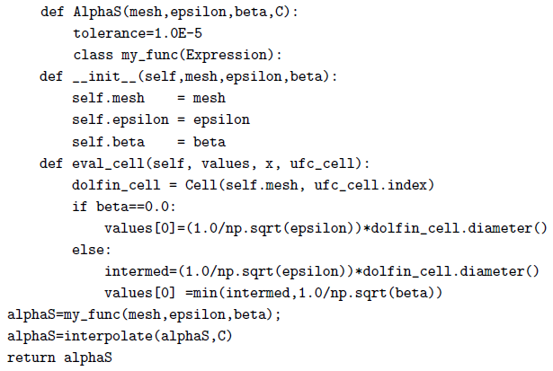
Parameter α _S was represented by means of a function over the same mesh and finite element space that was used to solve contaminant transport. Values were approximated by use of the cell diameter measures evaluated over all the cell indexes inside a FEniCS class . The error indicators were defined based on the residual expressions from previous presentation. For interior elements the α _S parameter was used as defined on the code that follows, however, edge elements consider that the operator avg (·), available on FEniCS ¹ , provide an estimate. The code for the α _S parameter, as a function over the finite element mesh, is provided:

The temporal residual contributions were based on the solution of the auxiliary problem and on the same considerations above. Finally, the analytical solution, C _A , when available, was evaluated by means of numerical quadrature package QUADPACK, which is available in SciPy ⁷ . To compare analytical and numerical values at nodal points the array format available in NumPy, ¹³ , was used. The graphical results were presented using Matplotlib ⁶ .

5 APPLICATION

5.1 Small advection with constant data

This section consider the contaminant transport equation on a rectangular domain $\Omega =(x_0,x_1)\times (y_0,y_1)=(0.0,3000.0)\times (0.0,1500.0)$ and is an adaptation from the problem presented in ¹⁰ . The physical parameters are $D_x=100.0\frac{{\displaystyle m^2}}{{\displaystyle d}},D_y=20.0\frac{{\displaystyle m^2}}{{\displaystyle d}}$ for longitudinal and transversal dispersion, $v_x=0.2\frac{{\displaystyle m}}{{\displaystyle d}}$ and $v_y=0.0\frac{{\displaystyle m}}{{\displaystyle d}}$ for velocity components and constant reaction $\lambda =0\in \mathrm{ℝ}$ .

The Figure 1 provides a graphical view of the domain Ω, the boundaries Γ_D and Γ_N , the velocity field, the function over the Dirichlet boundary and the initial condition. The Dirichlet boundary is on ${\Gamma }_D=\left\{x_0\right\}\times [y_0,y_1]$ and the expression (5.1) provides the normalized concentration function.

$C(x,y,t)=\left\{\begin{array}{cc}1.0,& \text{for}x=0,|y-750.0|<115.0,t>0\\ 0& \text{otherwise}\end{array}\right.$ (5.1)

Figure 1:
The domain Ω, the Dirichlet boundary Γ_D , the Neumann boundary Γ_N and the function C at $x=0$ .

Neumann boundary is on ${\Gamma }_N=\Gamma \setminus {\Gamma }_D$ with $g=n·\nabla \left(C\right)$ . The initial condition is $C(x,y,t_0=0)=0$ for all $x\in \Omega$ .

The Figure 2 shows the normalized concentration function $C=C(x,y,t)$ , the profiles and the level curves for finite element approximation with $n_x=2n_y=300$ triangular elements in each direction and left/right orientation, lagrangian linear functions, $\theta =1$ , time step $\tau =2.50d,t_{final}=1000.0d$ .

Figure 2:
Numerical solution, level curves and profiles in X,Y directions.

The numerical results are compared with the analytical solution for aquifer with infinite width and finite-width solute source given by the expression (5.2). A more detailed discussion and further references are available at ¹⁶ .

$$\begin{gathered} \begin{array}{l}{C}_A(x,y,t)=\frac{x}{\sqrt{\pi D_x}}\exp \left(\frac{xV}{2D_x}\right){\int }_0^{t/4}\frac{1}{Z^3}\exp \left(-\alpha Z^4-\frac{x^2}{4D_x{Z}^4}\right)\times \end{array} \\ \left[erfc\left(\frac{{\displaystyle Y_1-y}}{{\displaystyle 2Z^2\sqrt{D_y}}}\right)-erfc\left(\frac{{\displaystyle Y_2-y}}{{\displaystyle 2·Z^2\sqrt{D_y}}}\right)\right]dZ \end{gathered}$$ (5.2)

where $erfc(·)=1-erf(·)$ and erf (·) is the error function, $\alpha =V^2/4D_x+\lambda ,V=v_x$ is the velocity, Y ₁ and Y ₂ the lower and upper limits of contaminant source at $x=0$ , respectively.

The Figure 3 illustrates the error function $E=\left|C_A\right(x,y,t)-C(x,y,t\left)\right|$ at specific time of simulation process.

Figure 3:
Error function, level curves and profiles in X,Y directions.

It can be observed that the biggest error occurs in the discontinuity of the boundary function which is a result finite element mesh approximation using continuous functions. It is also observed that the magnitude of the error decreases rapidly with the distance from the points of discontinuity and that the advances of contaminant front is much smaller than the error due to discontinuity.

A direct calculation provides that $\epsilon =4$ and $\beta =0.0$ . Due to small value of velocity field, small advection governs groundwater flow. The spatial residual $\left(\right(\eta +\Theta {)}_{KE}={\eta }_{KE})$ indicator, the residual indicator due to element $\left(\right(\eta +\Theta {)}_K)$ and residual due to edge $\left(\right(\eta +\Theta {)}_E)$ are presented in Figures 4 , 5 and 6 , respectively.

Figure 4:
Spatial error indicator, level curves and profiles in X,Y directions.

Figure 5:
Element error, level curves and profiles in X,Y directions.

Figure 6:
Jump error indicator, level curves and profiles in X,Y directions.

The element and jump indicators capture the region of discontinuity, but there is a drastic variation in the magnitude of the estimates. In both cases, the indicators advance with a plume of contamination, but the magnitude of the estimates in the discontinuity region exceeds any of the other estimates in the finite element mesh.

From the joint analysis of the indicators, the dominance of the jump indicators over the indicators of the elements in the composition of the spatial indicator can be concluded. This dominance is accentuated around the points of discontinuity and the magnitude of dominance varies over the finite element mesh. This dominance, expressed locally by means of the relationship between the indicators, is reflected in the global estimates as presented in ¹² .

A more detailed view of the relationship between the residual indicators and the error function, around the points of greatest variation of error function can be obtained by analyzing the results presented in the Table 1 . In this table are the values of the nodes from finite element mesh, the values from of the numerical and analytical solutions, the error and the indicators for a set of points such that $E>0.5\max \left(E\right)$ . Due to the maximum value of the order $O\left({10}^{-}5\right)({\eta }_{\tau ,max}=3.58·{10}^{-05})$ , the temporal indicator was considered insignificant in this scenario and was disregarded from the analysis.

Table 1:
The numerical solution and the analytical solution for infinite domain with finite width font, the real error and error indicators for a set of points such that $E>0.5\max \left(E\right)$ .

( x, y )	C	C A	E	$(\eta +\Theta {)}_{KE}$	$(\eta +\Theta {)}_K$	$(\eta +\Theta {)}_E$
(10.0,630.0)	0.1955	0.2240	0.0286	7.3409	0.0499	7.3407
(20.0,630.0)	0.2953	0.3233	0.0279	3.9684	0.0237	3.9683
(30.0,630.0)	0.3479	0.3660	0.0181	3.0211	0.0178	3.0211
(10.0,640.0)	0.7934	0.7644	0.0290	6.9242	0.0499	6.9240
(20.0,640.0)	0.6816	0.6535	0.0281	4.0881	0.0286	4.0880
(30.0,640.0)	0.6171	0.5988	0.0183	2.5756	0.0178	2.5755
(10.0,860.0)	0.7934	0.7644	0.0290	7.3409	0.0499	7.3407
(20.0,860.0)	0.6816	0.6535	0.0281	3.9684	0.0237	3.9683
(30.0,860.0)	0.6171	0.5988	0.0183	3.0211	0.0178	3.0211
(10.0,870.0)	0.1955	0.2240	0.0286	4.5142	0.0305	4.5141
(20.0,870.0)	0.2953	0.3233	0.0279	3.5722	0.0237	3.5721
(30.0,870.0)	0.3479	0.3660	0.0181	2.7178	0.0176	2.7178

As final results, Figure 7 presents the profiles of the differences and the profiles of the indicators for a distinct set of finite element meshes. The analysis indicates that $n_x=300=2n_y$ provides more accurate solutions than the other meshes. Qualitatively, the residual indicators decrease in value as the number of elements in the meshes increases, as long as the time step is kept constant. In addition, the indicators preserve the dominance of the jump indicators over the element indicators. Finally, it was observed that the temporal indicators have a qualitative behavior that resembles the element indicator, shown in Figure 7-c , however, but with both different order of magnitude and maximum values.

Figure 7:
Profiles for a series of meshes with $n_x=200,250,300$ and $n_x=400$ at specific time. Profile for error function evaluated at $y=530$ and profiles for error indicators evaluated at $y=300$ .

5.2 Large advection with non-constant data

This example is an adaptation from the problem presented in ¹⁷ . The contaminant transport is defined on a rectangular domain $\Omega =(x_0,x_1)\times (y_0,y_1)$ with a variable velocity field $v=\left(v_x\right(x,y),v_y(x,y\left)\right)$ and a spatial dependence on the dispersion matrix $D=D(x,y)$ . The velocity field varies in both coordinated directions by means of linear mathematical relationship and the dispersion assumes a quadratic variation in principal components. Mathematically, the relations are:

$$\begin{gathered} v=(v_x,v_y)=(u_0·(x+1),-u_0·(y+1\left)\right) \\ D=\left[\begin{array}{cc}{d}_{xx}(x,y)& d_{xy}(x,y)\\ d_{yx}(x,y)& d_{yy}(x,y)\end{array}\right]=\left[\begin{array}{cc}{D}_0{u}_0^2·(x+1{)}^2& 0\\ 0& \begin{array}{c}{D}_0{u}_0^2·(y+1{)}^2\end{array}\end{array}\right] \end{gathered}$$

where u ₀ , D ₀ are constant values. The flow has a Dirichlet boundary with zero constant value at ${\Gamma }_D=\left\{x_0\right\}\times (y_0,y_1)\cup \left\{y_0\right\}\times (x_0,x_1)$ and a Neumann boundary on ${\Gamma }_N=\left\{x_1\right\}\times (y_0,y_1)\cup \left\{y_1\right\}\times (x_0,x_1)$ with values $g=n·D\nabla C$ . The source function was set to $f(x,y,t)=0$ and the initial condition was set to

$C(x,y,t=0)=\exp \left(-\frac{(x-{\mu }_1{)}^2}{2{\sigma }_1^2}-\frac{(y-{\mu }_2{)}^2}{2{\sigma }_2^2}\right).$

where µ ₁ , µ ₂ , σ ₁ and σ ₂ are constants. The Figure 8 is a schematic presentation of the domain with boundaries and initial concentration function.

Figure 8:
Schematic representation of domain, velocity field, initial condition, Dirichlet and Neumann boundaries.

The Figure 9 shows the concentration function $C=C(x,y,t)$ , the profiles and the level curves for finite element approximation with $n_x=n_y=200$ triangular elements in each direction and le ft / right orientation, lagrangian linear functions, $\theta =1/2$ , time step $\tau =.001,t_{final}=2.50,{\mu }_1={\mu }_2=5$ and ${\sigma }_1={\sigma }_2=0.5$ .

Figure 9:
Numerical solution, level curves and profiles in X, and Y directions.

Unlike the previous case, analytical solution are not available, both the dispersion and velocity data are space dependent functions and the flow is considered to be under large advection dominance. In this case, it is appropriate to use residual error indicators to access the quality of the numerical solution obtained using the finite element method.

The spatial residual indicator, $\left(\right(\eta +\Theta {)}_{KE})$ , the residual indicator due to element, $\left(\right(\eta +\Theta {)}_K)$ , residual due to edge, $\left(\right(\eta +\Theta {)}_E)$ and temporal indicator, ( η _τ ) are presented in Figures 10 , 11 , 12 and 13 , respectively. The spatial residual indicator is composed of the estimates of the elements, jumps and respective data contributions. This could be partitioned into the contributions of elements and jumps, but it was conveniently incorporated into spatial estimates. The temporal indicator, in turn, adds the solution of the diffusive problem to the temporal estimates of the small advection regime.

Figure 10:
Spatial error indicator, level curves and profiles in X, and Y directions.

Figure 11:
Element indicator, level curves and profiles in X, and Y directions.

Figure 12:
Edge indicator, level curves and profiles in X, and Y directions.

Figure 13:
Temporal error indicator, level curves and profiles in X, and Y directions.

Analogously to the previous case, the joint analysis of the results shows the predominance of jump indicators. Now the dominance was accentuated around the points of maximum value of initial condition function. However, it can be argued that, due to the smoothness of the data, the finite element mesh provides an appropriate representation for the data and, as a result, the indicators do not vary sharply as in the previous case. Despite this, the representation of the data in the finite space is not exact and introduces residual estimates due to the data approximation.

In this scenario, the residual temporal estimates, Figure 13 , and the residual estimates of the elements are of same order of magnitude and, therefore, cannot be ignored. However, the variations are more oscillatory and it can be seen that the maximum values occur in the same region where the maximums of the other estimates occur. It can be argued that spatial approximation has a strong influence on the temporal estimates due to diffusion associated problem, but a more detailed investigation was necessary.

A more detailed view of the relationship between the residual indicators can be obtained by analyzing the results presented in the Table 2 . In this table, are a few values of the numerical solution and error indicators such $C>0.975·\max \left(C\right)$ . The analysis and comparisons of these results provides an better understanding of the relationship between the error indicators: maximum values for spatial and edge indicators are of order O (10⁻⁰²) and order of maximum value for element indicator is O (10⁻⁰³), which is one order greater than the temporal indicator. It evidences that around the maximum values of concentration, temporal indicators has a smaller importance.

Table 2:
The numerical solution and the error indicators for a set of points such that $C>0.975·\max \left(C\right)$ .

( x, y )	C	$(\eta +\Theta {)}_{KE}$	$(\eta +\Theta {)}_K$	$(\eta +\Theta {)}_E$	η τ
(4.9,4.0)	0.0640	0.0333	0.0087	0.0321	0.0005
(5.0,4.0)	0.0640	0.0338	0.0086	0.0327	0.0008
(4.7,4.1)	0.0643	0.0231	0.0088	0.0213	0.0009
(4.8,4.1)	0.0646	0.0304	0.0088	0.0291	0.0006
(4.9,4.1)	0.0648	0.0212	0.0088	0.0193	0.0009
(5.0,4.1)	0.0648	0.0229	0.0087	0.0212	0.0005
(5.1,4.1)	0.0646	0.0328	0.0086	0.0316	0.0008
(5.2,4.1)	0.0642	0.0290	0.0084	0.0278	0.0005
(4.6,4.2)	0.0643	0.0277	0.0088	0.0262	0.0009
(4.7,4.2)	0.0648	0.0299	0.0088	0.0286	0.0006

Similar to Figure 7 , the behavior of residual indicators for successive refinements of finite element meshes is shown in Figures 14 and 15 . In the same way as in the previous case, the residual values decrease for successive refinements as long as the time step is kept constant. It should be noted that the time indicators now have the same order of magnitude as the element indicators and that, in addition, they still maintain a similar qualitative behavior.

Figure 14:
Spatial and element indicators profiles, at $y=4$ , for a series of meshes with $n_x=100,200$ and $n_x=300$ at specific time.

Figure 15:
Jump and temporal indicators profiles, at $y=4$ , for a series of meshes with $n_x=100,200$ and $n_x=300$ at specific time.

6 CONCLUSIONS

The presentation of the indicators as a surface over the finite element mesh provides an insight into the influence of contributions on the global estimator and the magnitude of relationships between the various individual contributions. The availability of the analytical solution allows to obtain a broader view of the behavior of the residual estimator and to infer the strict dependence between the residual estimates, the finite element mesh and the temporal partition. The mesh’s inability to capture abrupt variations in the data was reflected in the residual indicators and, as a logical consequence, in the residual estimates. In the case where the data is non-constant and smooth, the finite element space adequately captures the variations, but the data representation errors are inserted and must be taken into account when calculating the estimates or indicators. The dominance of advective processes increases the computational work to obtain residual estimates associated with the temporal partition in relation to the problems with dispersive dominance. In both cases, advective or dispersive dominance, the surfaces can be used to access the regions of greatest variation and define components that do not have significant contributions to the estimates. In addition, it is possible to monitor the variations in the surfaces of the indicators associated with the evolution of the contaminant distribution function.

REFERENCES

• ¹
  Fenics Project documentation. Available at https://fenicsproject.org/docs/dolfin/1.6.0/python/ .
  » https://fenicsproject.org/docs/dolfin/1.6.0/python/
• ²
  V. Batu. “Applied Flow and Solute Transport Modeling in Aquifers: Fundamental Principles and Analytical and Numerical Methods”. CRC Press Taylor (2006).
• ³
  J. Bear. “Hydraulics of Groundwater”. Dover Publications, Inc. (1979), 569 pp.
• ⁴
  S. Brenner & L. Scott. The Mathematical Theory of Finite Element Methods. In “Texts in Applied Mathematics, v. 15”. Springer-Verlag, New York (1994).
• ⁵
  R.E. Ewing. A posteriori error estimation. Computer Methods in Applied Mechanics and Engineering, 82(1-3) (1990), 59-72. doi:10.1016/0045-7825(90)90158-I. URL http://www.sciencedirect. com/science/article/pii/004578259090158I .
  » https://doi.org/10.1016/0045-7825(90)90158-I» http://www.sciencedirect. com/science/article/pii/004578259090158I
• ⁶
  J.D. Hunter. Matplotlib: A 2D graphics environment. Computing In Science & Engineering, 9(3) (2007), 90 -95.
• ⁷
  E. Jones, T. Oliphant, P. Peterson et al. SciPy: Open source scientific tools for Python (2001). URL http://www.scipy.org/ .
  » http://www.scipy.org/
• ⁸
  A. Logg. Automating the Finite Element Method. Archives of Computational Methods in Engineering, 14(2) (2007), 93-138. doi:10.1007/s11831-007-9003-9.
  » https://doi.org/10.1007/s11831-007-9003-9
• ⁹
  A. Logg, K.A. Mardal, G.N. Wells et al. “Automated Solution of Differential Equations by the Finite Element Method”. Springer (2012). doi:10.1007/978-3-642-23099-8.
  » https://doi.org/10.1007/978-3-642-23099-8
• ¹⁰
  G. Pinder. A Galerkin-finite element simulation of groundwater contamination on Long Island. Water Resources Research, 9(6) (1973), 1657-1669.
• ¹¹
  D. Praetorius, E. Weinmuller & P. Wissgott. A Space-Time Adaptive Algorithm for Linear Parabolic Problems. Asc report 07/2008, Institute for Analysis and Scientific Computing Vienna University of Technology - TU Wien (2008). Available at www.asc.tuwien.ac.at ISBN 978-3-902627-00-1.
  » www.asc.tuwien.ac.at
• ¹²
  J. Santos, A. Firmiano & E. Wendland. Jump Dominance on the Contaminant Transport Residual Error Estimator. TEMA - Trends in Applied and Computational Mathematics, (1) (2014). doi: https://doi.org/10.5540/tema.2014.015.01.0037 .
  » https://doi.org/10.5540/tema.2014.015.01.0037
• ¹³
  S. van der Walt, S. Colbert & G. Varoquaux. The NumPy Array: A Structure for Efficient Numerical Computation. Computing in Science Engineering, 13(2) (2011), 22-30. doi:10.1109/MCSE.2011.37.
  » https://doi.org/10.1109/MCSE.2011.37
• ¹⁴
  R. Verfürth. A posteriori error estimates for linear parabolic equations (2004). Available at http://www.ruhr-uni-bochum.de/num1/files/reports/APEELPE.pdf .
  » http://www.ruhr-uni-bochum.de/num1/files/reports/APEELPE.pdf
• ¹⁵
  R. Verfürth. Adaptive Finite Element Methods: Lecture Notes Winter Term 2013/14 (2014). URL http://www.ruhr-uni-bochum.de/num1/files/lectures/AdaptiveFEM.pdf .
  » http://www.ruhr-uni-bochum.de/num1/files/lectures/AdaptiveFEM.pdf
• ¹⁶
  E. Wexler. Chapter B7: Applications of hydraulics analytical solutions for one-, two- and three- dimensional solute transport in groundwater systems with uniform flow. In “Techniques of Water Resources Investigations of the United State Geological Survey, Book 3: Applications to Hydraulics”. U.S. Geological Survey, Denver, USA (1992).
• ¹⁷
  C. Zoppou & J. Knight. Analytical solution of a spatially variable coefficient advection-diffusion equation in up to three dimensions. Applied Mathematical Modelling, 23(9) (1999), 667-685. doi: 10.1016/S0307-904X(99)00005-0. URL http://www.sciencedirect.com/science/article/ pii/S0307904X99000050 .
  » https://doi.org/10.1016/S0307-904X(99)00005-0» http://www.sciencedirect.com/science/article/ pii/S0307904X99000050

Publication Dates

• Publication in this collection
  06 Sept 2021
• Date of issue
  Jul-Sep 2021

History

• Received
  04 Mar 2020
• Accepted
  01 Feb 2021