Growth of the tambaqui Colossoma macropomum (Cuvier) (Characiformes: Characidae): which is the best model?

Crescimento do tambaqui Colossoma macropomum (Cuvier) (Characiformes: Characidae): qual é o melhor modelo?

Abstracts

In order to decide which is the best growth model for the tambaqui Colossoma macropomum Cuvier, 1818, we utilized 249 and 256 length-at-age ring readings in otholiths and scales respectively, for the same sample of individuals. The Schnute model was utilized and it is concluded that the Von Bertalanffy model is the most adequate for these data, because it proved highly stable for the data set, and only slightly sensitive to the initial values of the estimated parameters. The phi' values estimated from five different data sources presented a CV = 4.78%. The numerical discrepancies between these values are of not much concern due to the high negative correlation between k and L<FONT FACE=Symbol>¥</FONT> viz, so that when one of them increases, the other decreases and the final result in phi' remains nearly unchanged.

Tambaqui; Colossoma macropomum; fish growth; Schnute's model; Central Amazon; Brazil

Para determinar qual o modelo de crescimento que melhor se ajusta ao tambaqui Colossoma macropomum Cuvier, 1818, foram utilizados 249 e 256 observações de comprimento-idade obtidos por meio de leituras de anéis em otólitos e em escamas, respectivamente, para os mesmos indivíduos. Para tanto, foi utilizado o modelo de Schnute, modelo genérico em que vários modelos tradicionais de crescimento estão incluídos. Com esse procedimento constatou-se que o modelo de von Bertalanffy realmente é o mais adequado, pois se mostrou altamente estável para o conjunto de dados, sendo pouco sensível aos valores iniciais adotados para as estimativas dos parâmetros. Os valores de fi' estimados a partir de cinco conjuntos diferentes de dados apresentaram CV = 4.78%, o que não é preocupante, pois as discrepâncias numéricas entre esses valores são conseqüência da alta correlação negativa entre k e L<FONT FACE=Symbol>¥</FONT> , visto que quando um aumenta o outro diminui e o resultado final expresso por F' permanece praticamente inalterado.

Tambaqui; Colossoma macropomum; crescimento de peixes; modelo de Schnute; Amazônia Central; Brasil

Growth of the tambaqui Colossoma macropomum (Cuvier) (Characiformes: Characidae): which is the best model?

Crescimento do tambaqui Colossoma macropomum (Cuvier) (Characiformes: Characidae): qual é o melhor modelo?

Penna, M. A. H^I; Villacorta-Corrêa, M. A^II; Walter, T.^III ; Petrere-JR, M.^I

^IDepartamento de Ecologia, UNESP, C.P. 199, CEP 13506-900, Rio Claro, SP, Brazil

^IIFaculdade de Ciências Agrárias, UFAM, Departamento de Ciências Pesqueiras, Av. General Rodrigo Otávio Jordão Ramos, 3000, CEP 69077-000, Manaus, AM, Brazil

^IIIFundo Nacional do Meio Ambiente, FNMA, Esplanada dos Ministérios, Bloco B, 7 º andar, CEP 70068-900, Brasília, DF, Brazil

^{Correspondence to}

ABSTRACT

In order to decide which is the best growth model for the tambaqui Colossoma macropomum Cuvier, 1818, we utilized 249 and 256 length-at-age ring readings in otholiths and scales respectively, for the same sample of individuals. The Schnute model was utilized and it is concluded that the Von Bertalanffy model is the most adequate for these data, because it proved highly stable for the data set, and only slightly sensitive to the initial values of the estimated parameters. The F' values estimated from five different data sources presented a CV = 4.78%. The numerical discrepancies between these values are of not much concern due to the high negative correlation between k and L¥ viz, so that when one of them increases, the other decreases and the final result in F' remains nearly unchanged.

Key words: Tambaqui, Colossoma macropomum, fish growth, Schnute's model, Central Amazon, Brazil.

RESUMO

Para determinar qual o modelo de crescimento que melhor se ajusta ao tambaqui Colossoma macropomum Cuvier, 1818, foram utilizados 249 e 256 observações de comprimento-idade obtidos por meio de leituras de anéis em otólitos e em escamas, respectivamente, para os mesmos indivíduos. Para tanto, foi utilizado o modelo de Schnute, modelo genérico em que vários modelos tradicionais de crescimento estão incluídos. Com esse procedimento constatou-se que o modelo de von Bertalanffy realmente é o mais adequado, pois se mostrou altamente estável para o conjunto de dados, sendo pouco sensível aos valores iniciais adotados para as estimativas dos parâmetros. Os valores de F' estimados a partir de cinco conjuntos diferentes de dados apresentaram CV = 4.78%, o que não é preocupante, pois as discrepâncias numéricas entre esses valores são conseqüência da alta correlação negativa entre k e L¥ , visto que quando um aumenta o outro diminui e o resultado final expresso por F' permanece praticamente inalterado.

Palavras-chave: Tambaqui, Colossoma macropomum, crescimento de peixes, modelo de Schnute, Amazônia Central, Brasil.

INTRODUCTION

Classical fish stock management models rely heavily upon growth parameter estimates which if biased or based on inadequate model premises lead to wrong strategies. Since the classical von Bertalanffy growth model fits most of the length/weight-at-age data, it is adopted a priori. In this paper we critically examine its adequacy for describing the growth of the tambaqui Colossoma macropomum Cuvier, 1818, in the Central Amazon basin based on length-at-age data from otholiths and scales readings.

The tambaqui is the largest characin of South America. It may reach more than 1 m in total length and 45 kg in total weight in a specimen observed at the Guaporé river, municipality of Costa Marques (RO), in 1989 by M. Petrere Jr. At present it is difficult to find individuals above 85 cm (20 kg) in the fish markets of the Central Amazon (Araújo-Lima & Goulding, 1997).

The favorite habitat of the tambaqui is the white-water rivers of the basins of the Amazon and Orinoco rivers. Eventually it migrates from clear, black waters to feed in flooded forest areas (Goulding, 1979, 1980, 1981; Goulding & Carvalho, 1982; Araújo-Lima & Goulding, 1997). Juveniles live in restricted flooded areas for approximately 5 to 6 years. When adults, in spite of feeding periodically in the flooded forest, they rarely remain at the varzea lakes when these are separated in the dry season from the main river (Costa, 1998).

According to Villacorta-Corrêa & Saint-Paul (1999), the tambaqui reaches sexual maturity by the time it averages 61 cm SL (standard length) and attains approximately 5 years of age.

The reproductive period of the species ranges from September to February with total spawning synchronous with the water level.

The tambaqui presents a unique combination of molariform teeth, which are adapted for breaking hard seeds, and numerous prolonged branchial bristles used for zooplankton retention (Goulding & Carvalho, 1982). Juveniles (TL (total length) < 60 cm) in general are omnivorous, feeding on fruits, seeds, and zooplankton (Honda, 1974; Goulding, 1979, 1980; Goulding & Carvalho, 1982; Villacorta-Corrêa, 1997). The young can also filter phytoplankton, whereas the adults feed exclusively upon fruits, such as those of the palm tree jauarí (Astrocaryum january), and seeds, e.g., those of the rubber tree seeds (Hevea spruceana, H. brasiliensis), which makes this fish an important seed disperser (Araújo-Lima & Goulding, 1997).

At the end of the 70s, in the Manaus fish market the tambaqui was the most important fish sold (Petrere, 1978). Merona & Bittencourt (1988) showed that the catch began to fall in the middle of the 80s, and the tambaqui is now overfished (Isaac & Ruffino, 1996).

The main objective of this paper was to test using the Schnute (1981) generic growth model, because it is that which better adjusts to age-at-length data, and then to compare the estimates of the parameters L¥, k, and t₀ with those already obtained by Costa (1998), Villacorta-Corrêa (1997), Isaac & Ruffino (1996), and Petrere (1983).

MATERIAL AND METHODS

Data

The complete dataset used in the present work was extracted from Villacorta-Corrêa (1997) and Penna (1999) for readings of scales (n = 256) and otholith rings (n = 249), and measures of standard length (SL, cm) of a single group of individuals.

We will describe the von Bertalanffy (1938) and Schnute (1981) models to fulfil as nearly as possible the aim of this paper.

Models

The von Bertalanffy growth model

Probably, the most used model to describe the growth curve in fish is that of von Bertalanffy (1938). Due to such wide acceptance, its parameters have been incorporated into several fish stock assessment models.

The original von Bertalanffy equation is:

where:

t = time;

t₀ = nominal age at which the individual fish presents length zero;

L_t= length at the instant t;

L¥ = asymptotic length (theoretical mean maximum size that an individual can reach);

k = growth coefficient (describes the speed at which L¥ is reached).

The parameters k, L¥, and t_o can be estimated through non-linear regression, as will be seen further on.

A more general way to write the von Bertalanffy growth curve was given by Schnute (1981):

We may call the von Bertalanffy curve "Pütter number 1" when p = 1, and "Pütter number 2" when p = 3. For these p values, the model is referred to as the specific equation of von Bertalanffy; for other values of p, the model is called von Bertalanffy generalized equation (Ricker, 1979).

The Schnute growth model

Because there are several models proposed in the literature for adjusting growth curves, the problem is to find the most suitable one. Therefore, Schnute (1981) developed a generic model in which the traditional growth models are incorporated as particular cases. This model has four statistically stable parameters with biological meaning.

The original equation proposed by Schnute is:

where:

y_t= length or weight of an individual at age t;

t = age;

t₁ = predetermined age of a young individual;

t₂ = predetermined age of an old individual;

g₁ = length or weight of an individual at age t_1;

g₂ = length or weight of an individual at age t₂.

Depending on the values of a and b, the Schnute generic equation 3 may change. We can cite 3 specific cases:

Case 1: a ? 0 and b = 0

Case 2: a = 0 and b ? 0

Case 3: a = 0 and b = 0

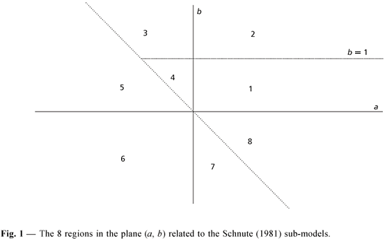
The parameters a and b describe the curve as being positive, negative, or zero. Parameter a is related to curve steepness (t^-1). Parameter b is dimensionless. A given combination of a and b indicates in which regions of Fig. 1 is the dataset, making it possible to determine which is the most appropriate sub-model.

Fig. 1

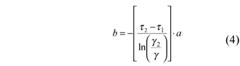
Fig. 2 presents the growth curves related to the possible Schnute sub-models.

Each one of the curves shown in Fig. 2 are related to the region of the same number in Fig. 1.

The following are some of the sub-models of Schnute method:

von Bertalanffy: included in regions (and respective curves) 1 (a > 0, 0 < b < 1) and 2 (a > 0, b = 1). Region 1 represents the classic situation in which all parameters are defined, corresponding to the von Bertalanffy model. The curve has an S shape and is asymptotic with the limit in g_oo(whose inflection point is located in (t*, y*), crossing the abscissa at age t₀). In region 2, the curve is asymptotic, crosses the axis t, with a non-existent inflection point.

Pütter number 1: located in region 2 (a > 0, b = 1) when b = 1;

Pütter number 2: located in region 1 (a > 0, b = 1) when b = 1/3 (a > 0, 0 < b < 1).

Other possible sub-models are: Richards, Gompertz, logistic, linear, quadratic, and exponential.

Table 1 shows all possibilities for each (a, b) combination related to the 8 regions of Fig. 1.

Applying the Schnute method

To apply Equation 3, initially we should choose initial values (seeds), with a certain number of observations, provided that they are not very close (for parameters g₁ and g₂ ), and pre-determine t₁ and t₂. Any current statistical package with a nonlinear program may simulate the data, using mean age classes for g₁ and g₂ (bearing in mind that g₁ > g₂), and whenever possible, the mean age should belong to the classes with the higher number of observations. It is important to remember that the mean ages only serve to predetermine parameters g₁ and g₂, and are not appropriate for data simulation. The initial a and b values can be obtained from the model that seems to be better adjusted to the data.

One can transform the parameters a and b of the Schnute model into conventional growth model parameters in the following way:

The parameters L¥ and t₀ depend on the observation pairs (a, b) for being calculated

(a ? 0, b ? 0):

(a ? 0, b = 0)

(a = 0, b ? 0)

Independent of a and b:

where:

y = theoretical maximum size;

t₀ = individual size at time zero;

t_* = projection of the curve inflection point in the abscissa;

y_* = projection of the curve inflection point in the ordinate;

z_* = increment rate at the curve inflection point.

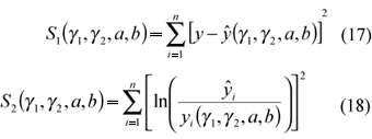
Error models

Schnute proposes two error models:

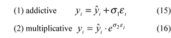
where:

e_i = random variable (i = 1, 2,..., n) considered independent and N(0,1);

s₁ = parameter which measures the addictive standard error (its unit depends on the unit measurement adopted);

s₂ = dimensionless parameter that measures the logarithmic standard error.

Their respective minimizing functions are:

Kimura maximum likelihood test

To test if two growth curves are different, a test of maximum likelihood developed by Kimura (1980) can be carried out. The Kimura equations are as follows:

where:

SQe + o = sum of the squared residuals of fitted curve to datasets 1 and 2;

SQe = sum of the squared residuals of the fitted curve to dataset 1;

SQo = sum of the squared residuals of the fitted curve to dataset 2;

n = total number of sampled individuals (n = n_otholiths + n_scales).

For sW, eight parameters are calculated and for s_w, four, giving us 4 degrees of freedom. Thus, Equation 18 follows an approximate c² distribution with 4 degrees of freedom.

F statistics

To test if the growth model indicated by Equation 3 is the most appropriate for the data, the following procedure should be followed (Schnute, 1981; Walter, 1997):

- Estimate the parameters g₁, g₂, a, and b, as described previously;

- verify the indicated region (Fig. 1) and estimate the 4 above parameters again, fixing b at the corresponding value for the region (Table 1), transforming the generic Schnute model (M_G) in a specific model (M₀);

- consider the sum of the squares of the residuals (SQ) of the two estimates;

- perform the hypothesis test:

H_O:M₀ is adequate to represent M_G; H₁:otherwise.

- To test this hypothesis, the Fisher distribution is used with (4-v, n-4) degrees of freedom:

where:

SQ₀ = sum of squares of the residuals of the specific model (M_O);

SQ_G = sum of squares of the residuals of the generic model (M_G);

v = number of parameters to be estimated;

n = number of individuals.

Growth performance index (Ö')

When fish growth is described by the same model, we can compare the growth performance between species or between stocks of the same species through F', which can be used to characterize species from a same family. Preliminary analyses suggest that F' coefficient of variation (CV) for several stocks of the same species should not exceed 5% (Gayanilo & Pauly, 1997).

The value of F' may be estimated by:

(according to Pauly & Munro, 1984)

RESULTS

The data were fitted by the generic equation of Schnute (Equation 3), using several combinations of the mean values of the datasets as initial values for g₁ and g₂. For the initial values of (a, b), (0,1) were used for both, because the von Bertalanffy equation is the one initially expected to better adjust to the data.

In Tables 2 and 3, we have the values of (a, b), SQ, g_1, and g₂, referent to the data of scales and otholiths, respectively, calculated by Equation 3 as well as the estimated values of the parameters k, L¥ and t₀, calculated by Equations (5), (6), and (7) respectively.

Fig. 3 shows the age-length graph for the scales data fitted by the Schnute model.

Fig. 4 presents the age-length graph for the otholith data, also fitted by the Schnute model.

To test if the von Bertalanffy model is the most appropriate, the parameters are again estimated fixing the value of b = 1. Equation (22) is used.

SQ_O (scales) = 888030.62 SQ_G (otholiths) = 509719.90

F_scales (1; 252) = 0.1132 P_scales = 0.737

F_otholits (1; 245) = 0.01895 P_otholiths = 0.89

In other words, M₀ for scales as well as for otholiths is appropriate to represent the generic model of Schnute. So, the values of L¥, k, and t₀ were calculated by Equations (5), (6) and (7), using the new values of a for scales and otholiths.

To test if the curves for otholiths and scales are different, the Kimura test was applied. Using Equations (20) and (21), we have:

SQe+o = 1397750.52; SQe = 887620.52;

SQo = 509681.58; n_otholiths + n_scales = 505

Inserting the appropriate values in the Equation (19), we have:

c ²(4) = 6.014; p = 0.198

Thus, we conclude that the curves for otholiths and scales are not statistically different.

DISCUSSION

The Schnute model, used in the present work, was shown to be highly stable for the dataset, and only slightly sensitive to the initial values of the estimated parameters. To test its robustness, several combinations of g₁, g_2,a, and b were used, as seen in Tables 1 and 2. It was also possible to prove that the model is highly stable (Walter, 1997).

In addition, through the method of Schnute it was possible to verify that the curve that better adjusts to the age-length data for the tambaqui is the von Bertalanffy growth equation (a > 0, b > 0). This is fortunate as Petrere (1983) and Isaac & Ruffino (1996), when estimating the MSY (maximum sustainable yield) for the tambaqui based on length-frequency distributions, adopted the Beverton & Holt (1957) model. This model is based on estimates of L¥ and k to which it is very sensitive. If we had shown that the von Bertalanffy growth model was not appropriate for the species, a drastic review of the practical consequences of these two papers would be necessary.

The difference between the values of L¥, k and t₀ for otholiths and scales probably is due to different results of ring counting in otholiths and scales.

Although widely employed, age determination in fishes through hard structures presents a series of difficulties when interpreting annual marks (Beamish, 1979; Carlander, 1990). Otholiths have been cited by several authors as more reliable for age determination, although Beamish & Chilton (1977) have argued that fin rays are more reliable for some fish species. Scale readings have the reputation of underestimating the true age, especially for older specimens (Campbell & Babaluk, 1979) and, therefore, it is recommended for young fish with high growth rates. Tropical fish marks are still considered difficult to interpret due to false rings, which may be mistaken for true rings (Casselman, 1983).

In the Table 5, the parameters L¥, k and t₀ are compared to those in the literature.

In our view the differences between our estimates and those of other authors may be due to:

(1) use of the Equations (6) and (7), instead of the linearized forms of the von Bertalanffy used in other research;

(2) Petrere (1983) and Isaac & Ruffino (1996) used length-frequency methods that are more subjective than ring readings;

(3) Costa (1998) fixed L¥ = 107.4 cm instead of estimating this parameter individually and, consequently, estimating k and t0 as a function of this L¥ value;

(4) Villacorta-Corrêa (1997) used retrocalculated lengths instead the original data. Although Villacorta-Corrêa (1997) did not

Although Villacorta-Corrêa (1997) did not conclude which of the reading methods is more reliable, we could argue that the estimates of L¥, k, and t₀ for otholiths would be more appropriate, because L_¥ = 100.4 cm is more plausible biologically than L_¥ = 85.12 for scales.

Besides, for otholiths the von Bertalanffy model is more appropriate, because when we fixed b = 1, its probability of being the most appropriate model was high.

Table 5 shows the F' values with a CV = 4.78%. In an analogy with a suggestion of Gayanilo & Pauly (1997), we could say that the numerical discrepancies between these values are not of much concern. This is due to the high correlation between k and L¥: when one of them increases, the other one decreases, and the final result in F' is nearly unchanged.

Acknowledgements — This work is a consequence of a Baccalaureate in Biological Sciences monograph presented by M. A. H. Penna, who was advised by M. Petrere Jr. to UNESP (Rio Claro).We thank INPA, UNESP, and CNPq for partially financing this research.

Received April 29, 2003 - Accepted July 8, 2003 - Distributed February 28, 2005

• ARAUJO-LIMA, C. & GOULDING, M., 1997, So fruitful a fish. Ecology, conservation, and aquaculture of the Amazon's Tambaqui Columbia University Press, New York, USA, 191p.
• BEAMISH, R. J., 1979, Differences in the age of Pacific hake (Merlucius productus) using whole otholiths and sections of otholiths. J. Fish. Res. Board Can., 36: 141-151.
• BEAMISH, R. J. & CHILTON, D., 1977, Age determination of lingcod (Ophiodon elongates) using dorsal fin rays and scales. J. Fish. Res. Board Can., 34: 1305-1313.
• BEVERTON, R. J. H. & HOLT, S. J., 1957, On the dynamics of exploited fish populations. U. K. Min. Agric. Fish., Fish Invest (Ser. 2), 19, 533p.
• CAMPBELL, J. S. & BABALUK, J. A., 1979, Age determination of walleye Stizosteidon vitreum (Mitchell), based on the examination of eight different structures. Can. Fish. Mar. Serv. Tech. Rep., 849: 23p.
• CARLANDER, K. D., 1990, A history of scale age and growth studies of North American freshwater fishes. In: R.C. Sommerfelt & G. E. Hall (eds.), Age and growth of fish Iowa State University Press, Iowa, pp. 3-14.
• CASSELMAN, J. P. M., 1983, Age and growth assessment of fish from their calcified structures: techniques and tools. In: L. M. Pulos (ed.), Proceedings of the International Workshop on Age Determination of Oceanic Pelagic Fishes: Tunas and Sharks NOAA Technical Report. National Marine Fisheries Service.
• COSTA, L. R. F., 1998, Subsídios ao Manejo do Tambaqui (Colossoma macropomum Cuvier,1818) na várzea do Médio Solimões: pesca, dinâmica de população, estimativa de densidade e dispersão MSc. Dissertation, INPA, Manaus, 76p.
• GAYANILO JR., F. C. & PAULY, D., 1997, The FAO-ICLARM stock assessment tools (fisat) user's Guide. FAO Computarized Information Series (Fisheries), 7: 124p.
• GOULDING, M., 1979, Ecologia da pesca do rio madeira CNPq/INPA, Manaus, 172p.
• GOULDING, M., 1980, The fishes and the forest: explorations in Amazonian natural history University of California Press, Berkeley, USA, 280p.
• GOULDING, M., 1981, Man and fisheries on an Amazon frontier The Hague: Dr. W. Junk Publishers. 137p.
• GOULDING, M. & CARVALHO, M. L., 1982, Life history and management of the tambaqui (Colossoma macropomum, Characidae): An important amazonian food fish. Revista Brasileira de Zoologia, 1: 107-133.
• HONDA, E. M. S., 1974, Contribuição ao conhecimento da biologia de peixes do Amazonas. II. Alimentação do tambaqui, Colossoma bidens (Spix). Acta Amazonica, 4: 47-53.
• ISAAC, V. J. & RUFFINO, M. L., 1996, Population dynamics of tambaqui, Colossoma macropomum Cuvier, in the lower Amazon, Brazil. Fisheries Management and Ecology, 3: 315-333.
• KIMURA, D. K., 1980, Likehood methods for the von Bertalanffy growth curve. Fishery Bulletin, 77(4): 765-776.
• MERONA, B. & BITTENCOURT, M. M., 1988, A pesca na Amazônia através dos desembarques no mercado de Manaus: resultados preliminares. Memoria Sociedad de Ciencias Naturales de La Salle, 48: 433-453.
• PAULY, D. & MUNRO, J. L., 1984, Once more on the comparison of growth in fish and invertebrates. ICLARM Fishbyte, 2(1): 21p.
• PENNA, M. A. H., 1999, Crescimento do tambaqui Colossoma macropomum Cuvier, 1818 (Characiformes: Characidae): qual é o melhor modelo? Baccalaureate in Biology Monograph, UNESP, Rio Claro (SP), 48p.
• PETRERE, M., 1978, Pesca e esforço de pesca no Estado do Amazonas. II. Locais, aparelhos de captura e estatísticas de desembarque. Acta Amazônica, 3: 1-54.
• PETRERE, M., 1983, Yield per recruit of the tambaqui, Colossoma macropomum Cuvier, in the Amazonas State, Brazil. Journal of Fish Biology, 22: 133-144.
• RICKER, W. E., 1979, Growth rates and models. In: W. S. Hoan & D. J. Randall (eds.), Fish physiology, bioenergetics and growth. Vol. 8. Academic Press, New York.
• SCHNUTE, J., 1981, A versatile growth model with statistically stable parameters. Canadian Journal of Fisheries and Aquatic Sciences, 38: 1128-1140.
• VILLACORTA-CORRÊA, M. A., 1997, Estudo de idade e crescimento do tambaqui Colossoma macropomum (Characiformes: Characidae) no Amazonas Central, pela análise de marcas sazonais nas estruturas mineralizadas e microestruturas nos otólitos Tese de Doutorado, Instituto Nacional de Pesquisas da Amazônia, Manaus, Amazonas, 217p.
• VILLACORTA-CORRÊA, M. A. & SAINT-PAUL, U., 1999, Structural index and sexual maturity of tambaqui Colossoma macropomum (Cuvier, 1818) (Characiformes: Characidae) in Central Amazon, Brazil. Rev. Bras. Biol., 59: 637-652.
• von BERTALANFFY, L., 1938, A quantitative theory of organic growth. Hum. Biol., 10: 181-213.
• WALTER, T., 1997, Curvas de crescimento aplicadas a organismos aquáticos Um estudo de caso para Toninha Pontoporia blainvillei (Cetacea, Pontoporiidae) do Extremo Sul do Brasil. Baccalaureate in Oceanography Monograph, FURG, Rio Grande, 101p.

Publication Dates

• Publication in this collection
  16 Nov 2005
• Date of issue
  Feb 2005

History

• Received
  29 Apr 2003
• Accepted
  08 July 2003