Tunneling Catastrophes of the Partition Function

Tunneling Catastrophes of the Partition Function

C. A. A. de Carvalho ^*

Instituto de Física, Universidade Federal do Rio de Janeiro,

Cx. Postal 68528, CEP 21945-970, Rio de Janeiro, RJ, Brasil

R. M. Cavalcanti⁺

Departamento de Física, Pontifícia Universidade Católica do Rio de Janeiro,

Cx. Postal 38071, CEP 22452-970, Rio de Janeiro, RJ, Brasil

Received April 29, 1997

We use path-integrals to derive a general expression for the semiclassical approximation to the partition function of a one-dimensional quantum-mechanical system. Our expression depends solely on ordinary integrals which involve the potential. For high temperatures, the semiclassical expression is dominated by single closed paths. As we lower the temperature, new closed paths may appear, including tunneling paths. The transition from single to multiple-path regime corresponds to well-defined catastrophes. Tunneling sets in whenever they occur. Our formula fully accounts for this feature.

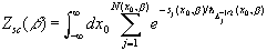
We may use path-integrals in the description of Quantum Statistical Mechanics. The partition function for a one-dimensional quantum-mechanical system, for instance, can be expressed as

,

(1)

.

(2)

For an arbitrary potential, V(x) , this integral has been approximated by means of perturbative [1,2], variational [1,2] and numerical [3] techniques. Here, we shall concentrate on the semiclassical approximation to the integral in order to: (i) derive a general formula for Z_sc(b) , for an arbitrary potential, that does not require a detailed knowledge of the classical motion; ^** (ii) discuss the onset of tunneling and relate it to the study of singularities in Catastrophe Theory.

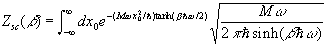
The semiclassical evaluation of (1) yields:

, (3)

where S_j(x₀,b) denotes the action and D_j(x₀,b) represents the determinant of the fluctuation operator,

, (4)

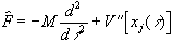both calculated at the j -th classical trajectory, x_j(t) , satisfying the boundary conditions ; N(x₀,b) is the number of classical trajectories which are minima of the action functional. (Note that x_j(t) are closed paths, but not necessarily periodic. If the integral in (3) is evaluated using the saddle-point approximation, then only the latter must be considered [4]. However, there are situations in which this further approximation cannot be used, e.g., if V(x) = lx⁴.)

The action has a simple expression in terms of the turning points of the classical trajectory:

. (5)

Here, and x₊^j (x_-^j) are turning points to the right (left) of x₀ . The first term in (5) corresponds to the high-temperature limit of Z(b) , where the classical paths collapse to a point, i.e., ® x₀ . For motion in regions where the inverted potential is unbounded (hereafter called unbounded motion), n = 0 . For periodic motion, n counts the number of periods and the second term is absent. For bounded aperiodic motion, all terms are present. The last two terms will be negligible for potentials which vary little over a thermal wavelength, . However, by decreasing the temperature, quantum effects become important.

For trajectories having a single turning point (n = 0) , are given implicitly by

, (6)

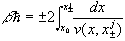and the fluctuation determinant by

. (7)

The formula above is only valid for trajectories with a single turning point ( n = 0 ). For those with two turning points, we have derived [5] a generalization which depends on the number of periods, n . However, the latter are naturally excluded from the calculation, as we shall see in the sequel.

Formulae (5) and (7) do not require full knowledge of the classical trajectory, as the dependence on x_j(t) comes only through the turning point. To see how this can simplify the evaluation of Z_sc(b), let us take the harmonic oscillator, , as an example. In this case, given x₀ and b there is only one trajectory, with a single turning point, given by for x₀ < 0 ( > 0) . S and D can also be readily calculated, the final result being

, (8)

which in this case is exact.

For , it is still true that there is only one trajectory, given x₀ and b, with a single turning point. Eq. (6) yields:

, (9) , (10) , (11)

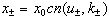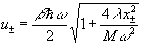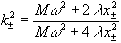where cn (u,k) is one of the Jacobian elliptic functions[6]. We may, then, use Eqs. (5) and (7), and change the integration variable in (3) from x₀ to x_± to obtain Z_sc(b) . The resulting integral can be evaluated numerically.

A more interesting situation occurs in the case of the anharmonic oscillator, V(x) = l(x ² - a ²)². For x ² > a ² only single paths with single turning points exist for fixed x₀ and b . However, there is also a region, x ² < a ², where the classical motion is bounded and a much richer structure exists[7], one in which more than one classical path may exist for given values of x₀ and b.

In a region of bounded classical motion (a well in - V ), such as x ² < a ² for the anharmonic oscillator, the number of classical trajectories changes as the temperature drops. If (where and x_m is a local minimum of - V ), for every x₀ in this region there is only one closed path, with a single turning point, satisfying the classical equations of motion. For x₀ < x_m (> x_m) this path goes to the left (right) and returns to x₀ . For x₀ = x_m , it sits still at the bottom of the well. It is this single-path regime which goes smoothly into the high-temperature limit.

For , the solution that sits still at x_m becomes unstable. Its fluctuation operator is that of a harmonic oscillator with w² = w²_m. Its finite temperature determinant is . This goes through zero at and becomes negative for , thus signaling that x(t) = x_m becomes unstable. At the same time, two new classical paths appear, symmetric with respect to x_m , as depicted in Fig. 1. Therefore, at x₀ = x_m, we go from a single-path regime to a triple-path regime as we cross . The two new paths are degenerate minima, whereas the path that sits still at x_m becomes a saddle-point of the action, with a single negative mode.

Figure 1. (a) Classical paths at x_m for (1) and (2 and 3); (b) Sketch of how the extrema change along the unstable direction in function space.

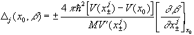
As b grows beyond , an analogous situation occurs for other values of x₀ inside the well. When the fluctuation determinant around the classical path for a given x₀ vanishes, a new classical path appears. Its single turning point lies opposite, with respect to x_m , to that of the formerly unique path. It may be interpreted as a tunneling trajectory, since it traverses a classically forbidden region of V . If b is increased further, this tunneling trajectory splits into two, as illustrated in Fig. 2. One is a local minimum of the action, whereas the other is a saddle-point, with only one negative mode. Again, we have transitioned from a single to a triple-path regime. As b grows, the triple-path region spreads out around x_m . The frontiers of that region are defined by the points x₀ such that .

Figure 2. (a) Classical paths at x_m for b < b_c (1), b = b_c (1 and 2&3) and b > b_c (1,2 and 3), < b_c <

2; (b) Sketch of how the extrema change along the unstable direction in function space.

The phenomenon just described is an example of catastrophe. It takes place whenever the number of classical trajectories changes, with one or more of them becoming unstable, as we lower the temperature. Conversely, we may say that the phenomenon is characterized by the coalescence of two or more of the classical trajectories, as we increase the temperature. This is akin to the ocurrence of caustics in Optics[8], where light rays play the role of classical trajectories and the action is replaced with the optical distance.

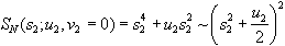
If we denote by s₁ the coordinate associated with the direction of instability of our example, the action can be viewed as S = S(s₁,...;x₀,b) . If we use the basis of eigenfunctions of the fluctuation operator around classical paths, s₁ will correspond to the direction along the one eigenfunction whose eigenvalue goes through zero, with the dots referring to all others. Catastrophe Theory[8,9,10] allows us to write down the "normal form'', S_N , of this generating function in the three-dimensional subspace made up by the unstable direction of state space (the set of paths) and the two control variables (related to b and x₀ ); it is this subspace which is relevant for the study of the onset of instability. As catastrophes are classified by their codimension in control space, which here is two-dimensional, only those of codimension 1 (the fold) or 2 (the cusp) are generic (i.e., structurally stable). The pattern of extrema then leads to the cusp, whose generating function is

S_N(s₁;u₁,v₁) = s₁⁴ + u₁s₁² + v₁s₁ , (12)

where u₁ and v₁ , the control parameters, are related to b and x₀ , respectively. This catastrophe is defined by

. (13)

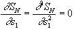Eliminating s₁ from these equations, we can draw the bifurcation set in control space (the curve ), as well as the pattern of extrema of S_N (Fig. 3). Assuming that u₁ and v₁ are linearly related to (b - ) and (x₀ - x_m) , respectively, for small values of both, we can also schematically plot the classical action (i.e., the action for classical trajectories) as a function of x₀ for different values of b;^*** see Fig. 4(a,b).

Figure 3. Bifurcation set for the cusp; pattern of extrema shown schematically.

Figure 4. Evolution of the classical action as b changes. (a)

; (b) < b < 2; (c) 2 < b < 3.

New tunnelings, accompanied by new catastrophes, will occur as we keep increasing b. From b = , we start having tunneling trajectories with , i.e., with one full period. For these, the determinant of fluctuations vanishes because the first, not the second bracket of (7) goes trough zero. However, the fluctuation operator around such tunneling trajectories already has a negative eigenmode. This follows from the fact that the zero-mode, given by , has a node. Thus, it cannot be the ground-state for the associated Schrödinger problem. This means that a new catastrophe takes place along a second direction in function space.

This new catastrophe is also a cusp. At x_m , as b becomes larger than 2, the solution that sits still acquires a second negative eigenvalue -- thus becoming unstable along a new direction in function space -- and two other solutions appear. They both have a negative eigenvalue along the first direction of instability and a positive eigenvalue along the new direction of instability. If we combine the information from both directions, we find that we go from two minima and a saddle-point with only one negative eigenvalue (hereafter, a one-saddle) to two minima, two one-saddles and one two-saddle. The two one-saddles are degenerate in action and represent time-reversed periodic paths. As b increases beyond 2, the same phenomenon takes place for x₀ around x_m : the one-saddles that already existed for b < 2in the three-path region around x_m become unstable along a second direction, and a five-path region grows around x_m , with two minima, two (periodic, degenerate in action) one-saddles and a two-saddle.

The new cusp can be cast into normal form using the second direction of instability:

. (14)

The absence of the linear term in Eq. (14) [compare with Eq. (12)] reflects the degeneracy in action of the two one-saddles. However, there is another degeneracy: since V does not depend on b, if x_cl(t) is a solution of the Euler-Lagrange equations, so is x_cl(t + t₀). If x_cl(t) is periodic, x_cl(t + t₀) describes the same path (and so has the same action), but with another starting point. This can be represented in Eq. (14) by the choice u₂a [(x₀ - x_m)² + k(2- b)] , with k > 0. See Fig. 4(c).

As we approach b = 3, the situation becomes similar to the one near b = . The difference is that we now have to deal with a tunneling path with more than one and less than two periods. Near b = 4, two-period tunnelings intervene, a situation similar to that at b = 2. The pattern which develops[11] is depicted in Fig. 5.

Figure 5. Partition of control space into p -solution regions (p = 1,3,5,7,...) .

Despite the fact that we keep adding new extrema as we lower the temperature, many of which represent tunneling solutions, only two of these are stable (i.e., minima). In a semiclassical approximation in euclidean time, appropriate to equilibrium situations, these are the only extrema we have to sum over, meaning that N(x₀, b) never exceeds two. The local minimum is a tunneling solution, whereas the global one becomes the unique solution in the high-temperature regime. For b > , there will be regions with either one or two minima of the classical action. The transition from a single-minimum to a double-minimum region occurs at values of x₀ where the fluctuation determinant vanishes due to the appearance of a caustic, thus leading to a singularity in the integrand of Eq. (3). This is not a disaster, however, as this singularity is integrable. (Such a singularity is an artifact of the semiclassical approximation. It disappears in a more refined approximation[8,12,13,14], in which one includes higher order fluctuations in the direction(s) of function space where the instability sets in.) We shall exhibit the details of this calculation in a forthcoming publication.

To conclude, two remarks: (i) our results may be used to derive a semiclassically improved perturbation expansion, which will be presented elsewhere; (ii) the semiclassical partition function incorporates, in an approximate way, quantum effects that become more and more relevant with the increase of the thermal wavelength. At very low temperatures, however, the quadratic approximations inherent to the semiclassical approximation fail to capture the details of the potential, which are important in the regime of large thermal wavelengths. Thus, we expect our calculations to be a better approximation at high temperatures. Indeed, studying the T = 0 limit of Z_sc(b) for the anharmonic oscillator, one finds no corrections to the unperturbed ground state energy. Nevertheless, this can be corrected by using the semiclassically improved perturbation theory just mentioned.

We thank Roberto Iengo, for useful conversations, Ildeu de Castro Moreira, for pointing out Ref. 9, Flavia Maximo, for help with the figures, and Moysés Nussenzveig and Alfredo Ozorio de Almeida, for a critical reading of this paper. Part of this work was carried out at the ICTP, and had financial support from CNPq, CAPES, FINEP and FUJB/UFRJ.

References

[1] R. P. Feynman and A. R. Hibbs, Quantum Mechanics and Path Integrals (McGraw-Hill, New York, 1965).

[2] R. P. Feynman, Statistical Mechanics (Benjamin, Reading, MA, 1972).

[3] M. Creutz and B. Freedman, Ann. Phys. (NY) 132, 427 (1981).

[4] See, for example, R. Rajaraman, Solitons and Instantons (North-Holland, Amsterdam, 1987), Sec. 6.3.

[5] To arrive at this result we adapted techniques described in: J. Zinn-Justin, Quantum Field Theory and Critical Phenomena (Oxford University Press, Oxford, 1993). A full derivation, together with explicit calculations for a number of potentials, will appear elsewhere.

[6] I. S. Gradshteyn and I.M. Ryzhik, Table of Integrals, Series and Products (Academic Press, New York, 1965).

[7] A partial examination of such a structure is found in: J. Ankerhold and H. Grabert, Physica A 188, 568 (1992); Phys. Rev. E 52, 4704 (1995); F. J. Weiper, J. Ankerhold and H. Grabert, Physica A 223, 193 (1996).

[8] M. Berry, in Physics of Defects, Les Houches Session XXXV (1980), eds. R. Balian et al. (North-Holland, Amsterdam, 1981); M. V. Berry and C. Upstill, in Progress in Optics XVIII, ed. by E. Wolf (North-Holland, Amsterdam, 1980).

[9] P. T. Saunders, An Introduction to Catastrophe Theory (Cambridge University Press, Cambridge, 1980).

[10] R. Thom, Structural Stability and Morphogenesis (Benjamin, Reading, MA, 1975); T. Poston and I. N. Stewart, Catastrophe Theory and its Applications (Pitman, London, 1978); E. C. Zeeman, Catastrophe Theory: Selected Papers 1972-1977 (Addison-Wesley, Reading, MA, 1977).

[11] This is an example of a sigma-decomposition. See, for example, M. Peixoto and R. Thom, C. R. Acad. Sc. Paris I, 303, 629 and 693 (1986); 307, 197 (1988) (Erratum); M. M. Peixoto and A. R. Silva, An. Acad. Bras. Ci. 62 (4), 321 (1990); M. M. Peixoto and A. R. Silva, preprint (1995).

[12] G. Dangelmayr and W. Veit, Ann. Phys. (NY) 118, 108 (1979).

[13] L. S. Schulman, Techniques and Applications of Path Integration (Wiley, New York, 1981).

[14] U. Weiss, Quantum Dissipative Systems (World Scientific, Singapore, 1993).

**

By classical motion we mean motion satisfying the Euler-Lagrange equation

, which is the equation of motion for a particle moving in a potential

minus

V

***

This plot can be obtained by exploiting the relation between the cusp and the swallowtail catastrophes. The latter has a generating function whose normal form is

, where

a ,

b ,

c are control variables. The extremum condition is, then,

. The identifications

will make the additional condition that defines the swallowtail,

, coincide with the requirement

. (In the jargon of catastrophe theory: the bifurcation set for the swallowtail coincides with the equilibrium hypersurface of the cusp.)

Publication Dates

• Publication in this collection
  04 Feb 1999
• Date of issue
  Sept 1997

History

• Received
  29 Apr 1997