Some limitations for the applicability of the ray method in elastodynamics

Algumas limitações à aplicabilidade do método do raio na elastodinâmica

Some limitations for the applicability of the ray method in elastodynamics

M. M. Popov¹ & S. Oliveira²

¹V. A. Steklov Mathematical Institute

Fontanka 27, 191011, St. Petersburg, Rússia.

²CPGG/UFBa, Rua Barão de Geremoaba s/nº

Instituto de Geociências, 40170-290, Salvador - Bahia

The ray method in the frequency domain describes the asymptotic behavior of the wave field for large frequencies which is not, in general, uniform with respect to the distance between the source and the point of observation. This implies that one can face situations in which the results obtained by the ray method may not be reliable for large distances from the source, if the dominant frequency is not high enough. In this paper we present two examples of such a type of problem for rather simple elastodynamic problems: a homogeneous medium; and a constant gradient velocity medium without interfaces. For both cases, the sources are assumed to be represented by two successive terms of the ray series, and therefore there are no point sources problems in our study. To this end we employ the following criterion of validity of the ray method: the absolute value of the ratio of the second term of the ray series to the first one must be less than unity. This criterion turns out to be sensitive to the radius of curvature of the initial wave front and to the initial distribution of the amplitude (or energy) along it. In the worst case of an initially planar wave front with nonuniform distribution of the amplitude, the second term of the ray series increases very fast. This gives rise to strong limitations to the use of the ray method with respect to distance if the frequency is fixed, or with respect to frequency for large distances. The depolarization phenomenon in both cases is discussed as well.

Key words: Ray method; Elastodynamics; Validity of asymptotics.

Algumas limitações à aplicabilidade do método do raio na elastodinâmica - O método do raio descreve o comportamento assintótico do campo de onda para altas freqüências. Em geral, este comportamento não é uniforme em relação à distância da fonte ao ponto de observação. Isto significa que este método pode fornecer resultados errôneos caso a freqüência dominante não seja suficientemente alta para calcular o campo a grandes distâncias da fonte. Neste trabalho são apresentados dois exemplos envolvendo problemas simples de propagação de ondas elásticas, onde o método do raio encontrou a citada dificuldade de aplicação. Estes exemplos envolvem um meio homogêneo e outro de gradiente constante de velocidade, ambos sem interfaces e onde consideramos o campo sendo gerado por uma frente de onda inicial e não por uma fonte pontual. Para chegar a este resultado, aqui foi aplicado o seguinte critério de validade da teoria do raio: o valor absoluto da razão entre o segundo termo da série do raio e o primeiro deve ser menor que a unidade. Tal critério é sensível ao raio de curvatura da frente de onda inicial e distribuição de amplitudes (ou energia) ao longo deste. O pior caso se refere a frente de onda inicialmente planar e com distribuição irregular de amplitudes. Neste caso, o segundo termo cresce muito rápido, implicando em severas limitações para o uso do método do raio com relação a distância à fonte, caso a freqüência seja fixada, ou com respeito à freqüência, se esta distância for muito grande. O fenômeno de despolarização também é discutido nos dois exemplos.

Palavras-chaves: Método do raio; Elastodinâmica; Validade da aproximação assintótica.

INTRODUCTION

In a number of geophysical applications, the ray method is used in situations when the dominant frequency of a wavelet is relatively small while the distance between the source and an observation point is large. Even if the characteristics of the inhomogeneous medium in such cases vary slowly as compared to the wavelength, the results obtained by the ray method may not be reliable. This conclusion follows from the fact that the ray method (as well as Maslov's and Gaussian beam methods) describes the asymptotic behavior for high frequencies, but are not uniform, in general, with respect to distance. On the other hand there are few examples in geophysics when the exact solution to elastodynamic wave propagation problems is available in closed analytical form. For instance the point source problems for an unbounded isotropic homogeneous medium as the center of dilation or rotation, and concentrated force in general (Aki & Richards, 1981). These solutions have the form of several terms of the ray series in 3-D and infinite asymptotic series for far field in 2-D. For example, in the case of the center of delatation in 3-D, it consists of two terms of the ray series. In fact, these solutions in the frequency domain depend on the product kr, where k is the wave number and r is the distance to the source. Therefore, asymptotics of the wave field for large k turns out to be uniform with respect to large r. Though these examples are very specific, they are exceptions in wave propagation theory, and tell nothing about more general cases. They give the idea that there are no limitations for the use of the ray method with respect to the distance to a source. If, however, one can find hints on the existence of such limitations in literature they are supposed to be caused by the variation of the velocity along rays. In other words, limitations may appear only in inhomogeneous media, see e.g. Cervený et al. (1977), page 204.

The main approach of this paper is to present some clarifying examples in which the ray method in elastodynamics faces serious limitations. For this aim we employ a criterion of validity of ray series suggested by Popov & Camerlynck (1996), and based on the theory of asymptotic series. According to this criterion we have to examine the absolute value of the ratio of the second term of the ray series to the first one. If this ratio is less than unity for given values of all the parameters of the problem, the main term can be used for approximation of the wave field; but not in the opposite case when the ratio is greater or equal to unity.

Unfortunately, this criterion is not easily applied, because the calculation of the second term of the ray series, though not very difficult in principle, requires cumbersome evaluations. Therefore we restrict ourservels to considerations of rather simple models for which the necessary calculations can be carried out almost analytically. Note that the problem of validity of the ray theory has been studied in the above mentioned paper by Popov & Camerlynck (1996) for the reduced wave equation in 2-D but also for more complicated models (wave-guide propagation).

In the first example we consider a 3-D homogeneous medium and assume that the initial wave field is given in the form of two terms of the ray series. The radius of curvature of the initial wave front is denoted by R and may vary in a wide range. Obviously, for an initially plane wave front R = ¥. The parameters involved are the following: radius of curvature R of initial wave front, distance to the point of observation, circular frequency w and distribution of the amplitude (or energy) along the initial wave front. We study the behavior of the second term as a function of these parameters. It turns out that, in the case of the plane wave front and non-uniform distribution of the initial amplitude along it, the second term increases proportionally with the distance to a point of observation. This strongly limits the use of the ray method with respect to distance if the dominant frequency is not large, or with respect to low values of frequency if the distance is large.

In the second example we consider a constant gradient velocity model without interfaces. Unfortunately, in this case we had to study a 2-D problem because of the extensive analytical calculations required. The parameters involved are the same as in the first example. It seems that here, the limitations to the ray method are even more severe in the case of an initially plane wave front and a nonuniform distribution of the amplitude along it.

We would like to emphasize that the two examples do not correspond to the point source problem mentioned above, in which the curvature of any wave front and the amplitude on it are strongly connected. In our examples both the curvature of the initial wave front and the amplitude on it are independent parameters. This is different to the problem considered by Vavrycuck & Yomogida (1995), and their formula for the second term of the ray series in the frequency domain can be obtained in our first example for particular values of these parameters. However, point source problems in inhomogeneous media are in broad use in geophysics and its applications, therefore it would be very interesting to check the validity condition of the ray method for those point source problems. Unfortunately, we face the caustic problem in the very beginning of such investigations because even in the vicinity of a point source, the integral in the expression for the second term of the ray series (see Eq. (6)) becomes singular. Thus, some, regularization procedure is required to compute the integral (Babich & Kirpichnikova, 1974). Then, in order to calculate the ray amplitudes on a given ray one needs to know rays which form a narrow ray tube centred on that ray, so the corresponding problem is actually local one. Therefore our results are valid for an arbitrary wave front which is locally spherical, i.e. is spherical in a vicinity of the given point on it. However, in general cases not only the curvature of the inicial wave front but also its derivatives influence on the second term of the ray series. We do not involve these derivatives into consideration as additional parameters of the problem in order to simplify calculations and because they will not change significantly the results obtained in this paper.

BASIC FORMULA OF THE RAY METHOD

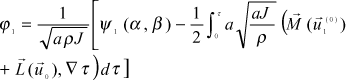
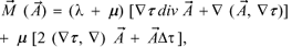
Consider a nonhomogeneous elastic medium with Lame's parameters l, m and density r. The ray series in the frequency domain is represented in the form

(1)

where means the displacement vector, is the amplitude vector and t is the eikonal. The main term corresponds to n = 0 and the second one to n = 1.

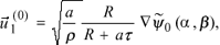
From here on we shall consider P-waves and for we have the following expressions

(2)

where,

is the velocity of P-waves, J is the geometrical spreading

and the function y₀ (a, b) of the ray parameters a, b describes the distribution of the amplitude along the initial wave front.

The second term has the form

(4)

where is orthogonal to Ñt and because of this it is called mixed term. It can be represented as follows

(5)

The expression for j₁ is more cumbersome

(6)

To complete the formulas for the second term, we must write down the expressions for the operators and . For an inhomogeneous isotropic medium in Cartesian coordinates, these formulas read

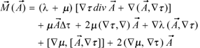
(7)

where stands for the double vector product, and

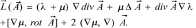
(8)

For details see Cervený et al. (1977), and original papers Karal & Keller (1959), and Alekseev et al. (1961).

Being rather cumbersome Eqs. (5) and (6) require special algorithms in order to apply them to geophysical models. An algorithm for computations of the second term has been suggested by Kirpichnikova et al. (1994).

EXAMPLE 1: HOMOGENEOUS MEDIUM

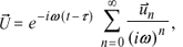
Suppose that the inicial wave field is given by two terms of the ray series with a spherical wave front of radius R centered at the point x₁ = -R, x₂ = x₃ = 0, see Fig. 1. We consider the central ray of a ray tube which coincides with x₁ axis and calculate the second term along this central ray. To this end we actually have to study rays from the ray tube around x₁ axis and do not need to know the global behaviour of the corresponding family of rays.

Figure 1 ¾
Initial wave front and ray parameters.
Figura 1 ¾ Frente de onda inicial e parâmetros do raio.

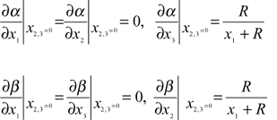
Let q and j be the angles of the spherical coordinates and let us introduce the ray parameters a and b by the following formulae

(9)

so that they have the sense of length along the initial wave front. Note that these parameters are suitable to study the uniform transition from the spherical initial wave front to the plane wave front, when R = ¥ and the angles of the spherical coordinates cannot be used as the ray parameters anymore.

Then, the corresponding family of rays as a function of the ray coordinates t, a, b takes the form

(10)

For the central ray of a ray tube we have q = 0, j = 0 and a = 0, b = 0. By substituting Eq. (10) into (3) we get the following expression for the geometrical spreading

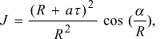
(11)

where the eikonal t can be regarded as a function of the coordinates x₁, x₂, x₃. Indeed, eliminating the ray parameters a and b in Eq. (10) we obtain

(12)

This allows us tho further simplify the calculations. By denoting we combine in Eq. (11) with an arbitrary function y₀ and present the function j₀in (2) in following form

(13)

which is more convenient for the following calculations.

Consider first the mixed term in Eq. (4). For homogeneous media it follows from (7), that

(14)

where we have to substitute A by j₀aÑt.

Employing Eqs. (9)-(14) we obtain for the mixed term

(15)

where the gradient of has to be calculated with respect to the coordinates x_i, i = 1, 2, 3. Therefore, to complete (15), we must regard as a compound function of x_i, i = 1, 2, 3 and the derivatives have to be computed on the central ray of the tube, i.e. on the x₁ axis. We deduce from Eqs. (10) the following result for the desired derivatives on the x₁ axis

(16)

Taking into account Eq. (16) we obtain the final expression for the mixed term on the central ray,

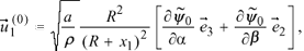
(17)

where by (j = 1, 2, 3) we denote the basis vectors of the Cartesian coordinates.

Consider further the function j₁ given by Eq. (6). We have to apply the operator in (14) to the mixed term (15) and the operator to . If follows from Eq. (8) that

(18)

Then, we have to calculate the scalar product on the central ray x₂ = x₃ = 0. Being not difficult in principle, the corresponding calculations turn out to be cumbersome. In order to reduce the size of the paper we omit them and confine ourselves to the following remarks for calculation.

1. In a homogeneous medium j₀ satisfies the transport equation

2 (Ñt, Ñj₀) + j₀Dt = 0,

which allows us to eliminate e.g. scalar product (Ñt, Ñj₀) in intermediate results.

2. By introducing the vector

we can present the eikonal t in (12) in the form

(19)

which seems to be useful in calculations. Using (19) one can, for instance, easily obtain

.

3. The function (a,b)depends on the ray parameters (9) and has to be regarded as the compound function of the coordinates (a (x₁, x₂, x₃), b (x₁, x₂, x₃)) in all intermediate calculations. It remains constant along each ray what implies that every ray belongs to a surface = k, for a certain constant value of k in the right-hand side. On the other hand, it is well known that Ñ is orthogonal to this surface and therefore Ñ is orthogonal to Ñt directed along the ray, i.e. (Ñ , Ñt) = 0. The latter identity provides simplifications in intermediate calculations.

4. In developing an expression with operator ( ) the following equality has to be taken into account:

(20)

The proof of Eq. (20) follows by differentiating Eq. (19),

(21)

Then,

(22)

Eq. (20) also provides simplifications.

Eventually, after some mathematics we arrive at the following result

(23)

where D means Laplace operator in coordinates x₁, x₂, x₃ applied to the function

In the last step we have to calculate the right-hand side of Eq. (23) on the central ray a = b = 0. Based on Eq. (10) we obtain

Further, using Eq. (16) we get

(24)

Employing Eqs. (11), (23), (24) we arrive at the following expression for j₁, given by Eq. (6), on the central ray x₁ = x₃ = 0 or a = b = 0:

(25)

where D_ab denotes the Laplace operator,

Apparently, for j₀ on the central ray we have

(26)

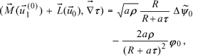
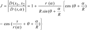
Note that, to apply the criterion of validity of the ray series we have to consider the ratio of the mixed term and of j₁ over j₀. So the multiplier R/(R + x₁) before brackets should not be taken into account.

Based on the Eqs. (17), (25) and (26) we arrive at the following conclusion.

If the distribution of the amplitude (or energy) along the wave front is uniform, i.e. y₀ does not depend on the ray parameters a, b, the mixed term vanishes. Depolarization phenomena does not exist in homogeneous media. From Eq. (25) for j₁ it follows that no serious limitations for the use of the ray method appear. Indeed, the dominant term in (25) tends to 1/R for large x₁ and does not increase. By means of moderate values of circular frequency w, the ratio can be kept less than unit for an arbitrary distance from the initial wave front.

Suppose now that the amplitude is not distributed uniformly along the initial wave front and that the derivatives of with respect to the ray parameters do not vanish. In this case we may observe a depolarization phenomenon, but its magnitude decreases with distance as 1/(x₁ + R)² and depends on the radius of curvature R of the initial wave front. In Eq. (25) for j₁ the last term dominates and for large distances it starts to depend upon R due to lim The criterion of validity of the ray series becomes sensitive to the radius of curvature of the initial wave front.

In the limiting case of an initially plane wave front (R = ¥) the situation changes drastically. The depolarization takes place and its magnitude remains independent of the distance x₁. But for j₁, we get in this case

(27)

and j₁ grows proportionally to the distance x₁ along the ray because Dabin the right-hand side of (27) is not equal to zero. This leads to strong limitations for the use of the ray method with respect to both distance and frequency. For large distances, we have to use high values of frequency in order to keep the ratio less than unity; and to study the depolarization phenomenon, we also have to take into account the first term of Eq. (4), which contains f₁ and essentially limits the validity of the ray method. Otherwise we can get wrong results in the case under consideration.

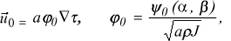
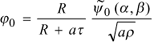
As an illustration of these results, the behavior of the ratio log where = aj₁Ñt as a function of the distance x₁ and the radius R of the initial wave front is depicted in Fig. 2. In the numerical computations we set a = 2500 m/s. For convenience we assume y₀, and y₁, along with the second derivatives of y₀, to be equal to one on the central ray under consideration, with a = b = 0. Though the latter option of y₀ and y₁ may seem to be artificial, it allows to demonstrate a trend in the behavior of this ratio. Of course, we could impose other values for y₀, y₁ and the derivatives of y₀ on the central ray, but it will not influence the trend of the curve on Fig. 2, what can be deduced from Eqs. (26) and (27). Notice that, in principle, a source of the wave field predetermines y₀ and y₁ as the function of the ray parameters but their finding in the particular case of the source may be a difficult task.

Figure 2 ¾
Evolution of log

EXAMPLE 2: CONSTANT GRADIENT VELOCITY MODEL

Consider a 2-D inhomogeneous elastic medium with the velocities a and b of the P and the S waves, respectively, given in the form a = a₁ + x₂a₂ and b = b₁ + x₂b₂. We suppose that the density r = 1 is constant and r = 1.

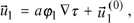
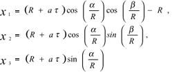
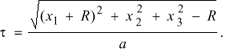
We assume that an initially cylindrical P-wave front with radius of curvature R passes the origin of the Cartesian system with coordinates x₁, x₂. The central ray of a ray tube starts from the origin under the angle p/2 ¾ q with the x₁ axis, see Fig. 3.

Each ray from a ray tube can be specified by the angle g, see Fig. 3, but instead of g we use a = gR as the ray parameter. The corresponding families of the rays can be presented in the form

(28)

where s is the arc length along the ray, r is the radius of curvature of the ray. It is well known that the rays are arcs of circles. Apparently, x₁ = x (a) and x₂ = z are coordinates of the centrum of the circle. Notice that z does not depend on the ray parameter.

Figure 3 ¾
Initial wave front and the ray parameters in 2-D case.
Figura 3 ¾ Frente de onda inicial e parâmetros do raio no caso 2-D.

For a = 0 we obtain the central ray of a ray tube, which starts from the origin for s = 0. This implies that x (0) = r (0) cos q and z = -r (0) sin q. All other rays from a ray tube start when s = 0 from the initial wave front given by the expression

(29)

Combining Eqs. (29) and (28) for s = 0 we arrive at the following formulas for r (a) and x (a).

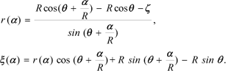
(30)

Thus, Eqs. (28) and (30) describe the desired family of rays, corresponding to the particular problem under consideration. In this case we used s and a as the ray coordinates instead of the eikonal t and a.

Eq. (2) for the main amplitude of the P-wave holds true in this case also, but the geometrical spreading (3) takes the form

(31)

In order to derive an expression for the mixed term we have to apply the operator to the main amplitude given by Eqs. (2) and (31). Though Eq. (7) for can be slightly simplified in the case under consideration, corresponding calculations turn out to be bulky. By introducing the unit vector orthogonal to the ray.

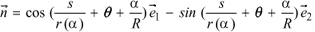
(32)

with , being base vectors of Cartesian coordinates, and after some algebric manipulations, the expression for the mixed term can be written down in the form

(33)

where Ñ means the gradient in Cartesian coordinates. It follows from Eq. (33) that the mixed term does not vanish in this case even if the distribution of the amplitude along the initial wave front is homogeneous, i.e. y₀ does not depend on a.

To develop an expression for j₁, defined by Eqs. (4) and (6), we had to use the software "Mathematica"and then to carry out the numerical calculations for the final results. In the computations we have used the following values for the velocities a = (2500 + 0.104x₂) m/s and b = (1750 + 0.073x₂) m/s. As in previous example, y₀, y₁ and the derivatives of y₀ with respect to the ray parameter were put equal to unity.

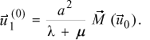
The evolution of log with distance along the central ray, fixed by is depicted in Fig. 4 for different values of the radius R of the initial wave front. In general, the behavior of the ratio is similar to the case of a homogeneous medium (compare with Fig. 2). Thus, in this example we also face the situation when restrictions for the use of the ray method appear with increasing distance to the initial wave front.

Figure 4 ¾
Same as Fig. (2) but for the constant gradient velocity model. The distance along the central ray is indicated on horizontal axis.
Figura 4 ¾ Gráfico correspondente ao da Fig. (2), mas para o meio com gradiente constante de velocidade. A distância ao longo do raio central é indicada no eixo horizontal.

We examine the depolarization phenomenon studying the absolute value of the ratio of the mixed term to the main term for non-homogeneous distribution of the amplitude along the initial wave front. The corresponding results are depicted in Fig. 5. For moderate values of R, the ratio declines with distance along the ray, while for large R and an initially planar wave front it remains almost independent of the distance. However, precisely in those cases the first item = aj Ñt of the second term (4) has to be taken into account due to its dominant role in the regulation of the applicability of the ray method itself.

Figure 5 ¾
Depolarization phenomen on. Evolution of log

CONCLUSION

It follows from the examples discussed above that serious restrictions to the ray method in elastodynamics may appear even for rather simple models. In the cases under consideration, the validity of the ray theory is sensitive to the distribution of the amplitude along the initial wave front and its radius of curvature. But are they the only parameters which strongly influence the behaviour of the second term of the ray series? The worst situation is observed for the initially planar wave front and a nonhomogeneous distribution of the amplitude along it. Even for small variations of the amplitude in the lateral directions the second term grows proportionally to the distance between the initial wave front and the point of observation. Thus, to keep the value of the ratio which regulates the applicability of the ray method, less than unity we have: either to increase the low limit of frequency with increasing distance, or if the frequency is bounded from above, to limit the value of the distance. We stress once again that for both examples the well-known validity conditions of the ray theory, such as small variations of the medium along a wavelength, and of a gradient of the amplitude compared to the amplitude itself are fulfilled. Nevertheless, the ray theory may be out of the range of its validity. This proves that being rather heuristical, those conditions cannot be regarded as sufficient and therefore reliable in every case.

We could and would like to suggest the following interpretation to these results.

If we consider the ray theory only to the first approximation, taking into account only the main term n = 0 of the ray series (1), we can construct a beam of the wave field which propagates along the central ray without spreading. The whole energy of the wave field will remain in this beam because the energy propagates along ray tubes and there are no transversal diffusion of it across the ray tubes.

Indeed, in the first example we have family of rays paralell to the x₁ axis originally emanated from the initial plane wave front. Varying the amplitude, exactly the function j₀, along the initial wavefront this ray field can be bounded in the lateral directions. To this end j₀ should be non-zero only in some domain on the initial wave front and then it has to be extended smoothly to zero values in the rest of the initial wavefront. Thus, the obtained wave beam does not spread in the lateral directions at all because the geometrical spreading is constant everywhere. The energy of the initial wave field will propagate with this beam without transversal diffusion, and no limitations with respect to the distance of propagation of this beam appear.

It is, however, apparent from the physical point of view and from experiments as well, that such view and from experiments as well, that such type of propagation phenomenon cannot exist. We know from mathematics that a source of finite geometrical dimensions gives rise to a spherical wave for large distances from it in 3-D, but not for the beam above described. Evidence for that exists also in the ray theory itself, but we have to take into account the second term n = 1 in the ray series (1). Exactly in this case the second term increases with distance what sets up a limitation for the existence of such a beam with respect to distance. Thus, we can conclude that the ray method fails in these particular cases because it does not describe properly the transversal diffusion of the energy of the wavefield.

It would perhaps be an exciting task just to check whether numerous applications of the ray theory in geophysics have been carried out in frames of the validity of the theory. Unfortunately, this task will require extensive studies of the second term of the ray series and developments of the corresponding computer codes.

ACKNOWLEDGMENTS

This research was supported by CNPq (Conselho Nacional de Desenvolvimento Científico e Tecnológico) and Petrobras (Petróleo Brasileiro S.A.) and partly (for M.P.) by Russian Fund of Fundamental Research N96-01-00666. We are thankful to Prof. E. Sampaio for critical reading the manuscript and to Prof. P. Hubral for discussions.

Submetido em: 05/11/97

Revisado pelo(s) autor(es) em: 09/05/98

Aceito em: 15/05/98

ALGUMAS LIMITAÇÕES À APLICABILIDADE DO MÉTODO DO RAIO NA ELASTODINÂMICA

O método do raio é uma ferramenta para estudos de propagação de onda largamente usado na sísmica e na sismologia. Este método é empregado particularmente em situações onde a velocidade do meio varia lentamente comparada com o comprimento de onda dominante e em que é necessário calcular o campo a uma grande distância, medida em comprimentos de onda, da fonte. Porém, mesmo se a velocidade variar muito suavemente, os resultados obtidos pelo método do raio podem não ser confiáveis para a situação descrita anteriormente. Esta conclusão é conseqüência de que o método do raio fornece resultados que são assintóticos com relação às altas freqüências, mas estes, em geral, não são uniformes com relação à distância. Contudo, na literatura, tais limitações à aplicabilidade deste método são estudadas à luz de critérios heurísticos, formulados em termos da variação da velocidade ao longo do raio e, portanto, aparentemente, só apareceriam em meios heterogêneos.

O objetivo deste trabalho é apresentar alguns exemplos esclarecedores nos quais o método do raio, aplicado à propagação de ondas elásticas, encontra sérias dificuldades. Para este propósito nós empregamos um critério de validade que é consistente com a teoria das séries assintóticas. De acordo com este critério, é necessário que se examine como se comporta a razão entre o segundo termo da série do raio com relação ao primeiro termo desta série. Se esta razão for menor que um, o primeiro e principal termo pode ser usado como uma aproximação do camp de onda. Caso esta razão seja maior que um, o termo principal não pode ser considerado uma aproximação válida para o campo. Infelizmente, este critério não é fácil de aplicar, pois a obtenção do segundo termo, embora simples em princípio, requer longos e tediosos cálculos. Devido a isto, nos restringimos a modelos simples, para os quais os cálculos puderam ser feitos quase todos analiticamente. Outra dificuldade aparece no caso de fontes pontuais. Para× estas, o cálculo do segundo termo requer regularização devido à singularidade que surge no local da fonte. Para evitar esta complicação extra, consideramos o campo sendo gerado a partir de uma frente de onda inicial.

No primeiro exemplo, foi considerado o problema do campo de ondas P sendo gerado por uma frente de onda inicial esférica em um meio homogêneo. O comportamento do segundo termo foi estudado com relação aos seguintes parâmetros: raio de curvatura R da frente de onda inicial, distância a um ponto de observação, freqüência angular w, e distribuição de amplitudes (ou energia) ao longo da frente de onda inicial. Neste exemplo, foi observado que, no caso da frente de onda inicialmente planar (R = ¥) com distribuição irregular de amplitudes, a componente de despolarização do segundo termo (que é ortogonal à direção de propagação) mantém-se independente da distância da frente de onda ao ponto de observação, ao passo que a componente do segundo termo, na direção de propagação, cresce proporcionalmente com a distância ao ponto de observação. Este fato limita fortemente o uso do método do raio com respeito à distância, se a freqüência não for suficientemente alta, ou com respeito a baixas freqüências, caso a distância da frente de onda ao ponto de observação seja grande. Este exemplo também deixa claro que limitações ao método do raio podem surgir até mesmo em meios homogêneos.

No segundo exemplo, nós consideramos um meio onde a velocidade é uma função linear da profundidade. Para minimizar os cálculos, nos restringimos ao caso 2-D, em que o campo é gerado por uma frente de onda inicial cilíndrica. Os parâmetros envolvidos foram os mesmos do primeiro exemplo, porém as limitações encontradas foram ainda mais severas. Em vista destes resultados, fica claro que é importante checar se as numerosas aplicações do método do raio estão de acordo com a validade da teoria. Esta tarefa requer o estudo intensivo do segundo termo da série do raio. Para isto, é necessário que se desenvolvam algoritmos eficientes para o cálculo deste termo.

NOTAS SOBRE OS AUTORES

NOTES ABOUT THE AUTHORS

ALGUMAS LIMITAÇÕES À APLICABILIDADE DO MÉTODO DO RAIO NA ELASTODINÂMICA - SOME LIMITATIONS FOR THE APPLICABILITY OF THE RAY METHOD IN ELASTODYNAMICS

Mikhail M. Popov

Professor in Steklov Mathematical Institute of St. Petersburg, Russia. He has a D.Sc degree in mathematical physics and has worked for decades in wave propagation and theory of difractions, including propagation of seismic waves. He is leading researcher in Steklov Mathematical institute of Academy of Sciences in Russia and has published over than 80 scientific papers. He was visiting professor in CPGG-UFBa during one semester in 1995 and 1996.

Sérgio A. M. Oliveira

Formou-se em Engenharia Elétrica pela Universidade Federal da Bahia em 1993. Obteve, em 1998, seu D.Sc. em Geofísica pelo Centro de Pesquisas em Geofísica e Geologia da UFBa. Suas áreas de interesse incluem propagação de ondas e métodos geofísicos para exploração de hidrocarbonetos.

CAMADAS NEUTRAS ESPORÁDICAS NA ALTA ATMOSFERA ASSOCIADAS COM ONDAS ATMOSFÉRICAS - WAVE ASSOCIATED SPORADIC NEUTRAL LAYERS IN THE UPPER ATMOSPHERE

Barclay Robert Clemesha

Bacharel em Física pela University of London em 1957. Em seguida trabalhou como pesquisador no Projeto denominado International Geophysical Year na University College Ibadan, Nigéria, por três anos, na área de física da baixa ionosfera. Transferiu-se então para a University of Ghana, Accra, onde trabalhou com pesquisas em irregularidades na região F da ionosfera. Em 1963 transferiu-se para a University of the West Indies, Kingston, Jamaica, onde juntamente com os Drs. Geoffrey Kent e Ray Wright desenvolveu um dos primeiros radares de laser para estudos atmosféricos. Completou seu Ph.D. na University of the West Indies em 1968. Desde o final de 1968 trabalha no Instituto Nacional de Pesquisas Espaciais (INPE) onde coordena o grupo de Pesquisas da Alta Atmosfera (FISAT). É membro do Comitê Editorial do periódico indexado Journal of Atmospheric and Terrestrial Physics (Pergamon - ISSN 0021-9169). É membro da Sociedade Brasileira de Geofísica e do American Geophysical Union (AGU), USA. Suas áreas de interesse atualmente incluem estudos da dinâmica e química da alta mesosfera e baixa termosfera usando radar de laser, medidas de aeroluminescência tomadas de solo e via experimentos com foguete.

Paulo Prado Batista

Bacharel em Física pela Universidade Federal de Goiás em 1972. Mestre e Doutor em Ciência Espacial pelo Instituto Nacional de Pesquisas Espaciais (INPE) em 1976 e 1983, respectivamente. Fez estágio de Pós-Doutorado por um ano na Universidade de Boston, USA, em 1987. Iniciou carreira no INPE em 1973 como Auxiliar de Pesquisas e onde continua até o momento como Pesquisador Titular. Suas áreas de interesse são: Dinâmica da média atmosfera, com ênfase em estudos de marés atmosféricas e ondas de gravidade na média atmosfera com medidas por meio de aerolumunescência , radar de laser e foguetes de sondagem. É membro da Sociedade Brasileira de Geofísica e da American Geophysical Union.

Dale Martin Simonich

Bacharel e mestre em Engenharia Elétrica pela Marquette University, Milwaukee WI, EUA em 1963 e 1965. Doutor em Engenharia Elétrica pela Universidade de Illinois at Urbana - Champaign, Urbana IL, EUA em 1972. Atualmente é Pesquisador Titular no Instituto Nacional de Pesquisas Espaciais - INPE responsável pelo projeto de radar de laser. Áreas de interesse: Estudos da dinâmica e química da mesosfera usando a técnica de radar de laser, aerossóis estratosféricos, e desenvolvimento de equipamentos e software para o radar de laser.

INFLUÊNCIA SELETIVA DA TURBULÊNCIA SOBRE AS ONDAS DE ROSSBY E DE LAMB NA ATMOSFERA BAROTRÓPICA - THE SELECTIVE INFLUENCE OF THE TURBULENCE ON THE ROSSBY AND LAMB WAVES IN THE BAROTROPIC ATMOSPHERE

Vladimir Kadyschnikov

Concluiu Mestrado em Mecância (1958) na Universidade de Moscou (Rússia), Doutorado (1964) em Geofísica no Observatório Principal de Geofísica em São Petersburgo, Pós-doutorado em Mecânica e Matemática (1985) no Centro Hidrometeorológico da Rússia em Moscou. Nos anos de 1990-1994 foi Chefe da Seção dos Métodos Numéricos da Previsão do Tempo de Curto Prazo neste Centro. Desde 1995 é Professor Adjunto do Curso de Pós-graduação em Meteorologia da Universidade Federal de Pelotas. Tem mais de 60 artigos publicados em periódicos russos. Área de especialização: Modelagem Numérica dos Processos Atmosféricos.

Darci Pegoraro Casarin

Graduado em Engenharia Eletrônica pela Universidade Federal do Rio Grande do Sul (1976), Mestre pelo Instituto de Pesquisas Espaciais (1982) com a dissertação entitulada "Sistemas de Bloqueio no Hemisfério Sul". É Professor da Universidade Federal de Pelotas -UFPEL desde 1979. Foi Diretor da Faculdade de Meteorologia da UFPEL no período 1989-1993 e Chefe do Centro de Pesquisas Meteorológicas da UFPEL até 1997.

• Aki, K. & Richards, P. G. - 1981 - Quantitative seismology. Freemen, New York.
• Alekseev, A. S., Babich,V. M. & Gelchinskii, B. Ya. - 1961 - Ray method calculations of intensity of wave fronts, problems of the dynamic theory of seismic wave propagation. Leningrad Univ. Press, 5: 3-24 (in Russian).
• Babich, V. M. & Kirpichnikova N. Ya. - 1974 - The Boundary Layer Method in Diffraction Problems, Leningrad State Univ., St. Petersburg, Russia (in Russian). English translation in Springer Series in Electronics 3, 1979.
• Cervený, V., Molotkov, I. A. & Psencík, I. - 1977 - Ray method in seismology. Univ. of Prague Press, Prague, Czech. Republic.
• Karal, F. G. & Keller, J. B. - 1959 - Elastic wave propagation in homogeneous and inhomogeneous media, JASA, 31: 394-405.
• Kirpichnikova, N. Ya., Popov, M. M. & Psencík, I. - 1994 - An algorithm for computation of the second term of the ray method series in an inhomogeneous isotropic medium. Zap. Nauchn. Semin. S.-Petesburg. Otdel. Mathem. Inst. V. A. Steklova, 210: 73-93 (in Russian, English transl. to appear in J. Math. Sciences).
• Kirpichnikova, N. Ya. & Popov, M. M. - 1994 - Computation of the second term of the ray method series in two and a half dimension. Zap. Nauchn. Semin. S.-Petersburg. Otdel. Mathem. Inst. V. a. Steklova, 210: 94-108 (in Russian, English transl. to appear in J. Math. Sciences).
• Popov, M. & Camerlynck, C. - 1996 - Second term of the ray series and validity of the ray theory, JGR, 101 (B1): 817-826.
• Vavrycuk V. & Yomogida K. - 1995 - Multipolar elastic fields in homogeneous isotropic media by high-order ray approximations, Geophys. J. Int. 121: 925-932.

Publication Dates

• Publication in this collection
  08 June 2001
• Date of issue
  Nov 1997

History

• Accepted
  15 May 1998
• Reviewed
  09 May 1998
• Received
  05 Nov 1997