FUZZY INFERENCE SYSTEMS FOR MULTI-STEP AHEAD DAILY INFLOW FORECASTING

ABSTRACT

This paper presents the evaluation of a daily inflow forecasting model using a tool that facilitates the analysis of mathematical models for hydroelectric plants. The model is based on a Fuzzy Inference System. An offline version of the Expectation Maximization algorithm is employed to adjust the model parameters. The tool integrates different inflow forecasting models into a single physical structure. It makes uniform and streamlines the management of data, prediction studies, and presentation of results. A case study is carried out using data from three Brazilian hydroelectric plants of the Parana basin, Tiete River, in southern Brazil. Their activities are coordinated by Operator of the National Electric System (ONS) and inspected by the National Agency for Electricity (ANEEL). The model is evaluated considering a multi-step ahead forecasting task. The graphs allow a comparison between observed and forecasted inflows. For statistical analysis, it is used the mean absolute percentage error, the root mean square error, the mean absolute error, and the mass curve coefficient. The results show an adequate performance of the model, leading to a promising alternative for daily inflow forecasting.

Keywords:
inflow forecasting; hydroelectric plants; fuzzy inference systems

1 INTRODUCTION

Hydroelectric operation planning is important even in countries with wide availability of water resources. For example, Brazil has more than 140 hydroelectric plants that contribute almost 80% of its power generation capacity. Despite the large hydroelectric potential, in 2001 thereservoir levels decreased and forced the Brazilian population to reduce their energy consumption (^{ANEEL, 2008}).

In this context, an important activity is the inflow forecast. It is fundamental to the planning of the water and energy resources of a system. It is important to have accurate estimates of the variables involved in the hydroelectric planning so that computational models, used for optimization and simulation of the system, provide reliable results (^{Hidalgo et al., 2012}, ²⁰¹⁴; ^{ONS, 2010};^{Lopes, 2007}).

A considerable amount of research has been conducted in order to formulate models that aim to improve the quality of the predicted inflows. In general, these models are assigned to one of two broad categories: conceptual or parametric.

Conceptual models require a large amount of high-quality data associated with geographical, hydrological, and meteorological characteristics. Parametric models use mathematical functions to relate meteorological variables to inflow (^{Coulibaly et al., 2005}; ^{Dawson & Wilby, 2001}). They do not require a detailed understanding of the basin’s physical characteristics (^{Zhang et al., 2009}).

Regarding the used technique, the models can be deterministic, stochastics, statistics, neural networks or fuzzy systems. Soil Moisture Accounting Procedure (SMAP) is an example of deterministic conceptual model. It considers the basin’s physical processes to represent the variables (^{Lopes et al., 1982}). Stochastic models employ the concept of probability for occurrence of the inflows. As example can be cited the linear stochastic model named MEL (^{ANEEL, 2007}). Linear regression is a statistic technique used in some researches, such as in (^{Souza Filho & Lall, 2004}).

Neural networks and fuzzy systems are versatile tools as they can be applied to several time series problems. They are employed in situations where it is difficult to determine the physical process or when it is not possible to obtain a mathematical representation of the process (^{Bowden et al., 2005}). They always yield some answer even when the input information is not complete. Neural Networks and fuzzy systems models can process non-linear problems and complex data. Therefore, they are interesting for forecasting of hydrological data.

In (^{D’Angelo et al., 2011}) a Kohonen neural network is used to find the best centers of time series to be used in fuzzyfication process; in (^{Melo et al., 2007}) it is applied to predict the daily and monthly sugar price. (^{Wong et al., 2010}) present a novel adaptive neural network to predict periodical time series with a complicated structure.

Concerning inflow forecasting, (^{Nayak et al., 2004}) present the application of an Adaptive Neuro Fuzzy Inference System (ANFIS) for modeling of hydrologic time series. The results show that the forecasted flow series preserve the statistical properties of the original flow series.

(^{Bravo et al., 2009}) present the performance of two medium-range streamflow forecast models: a multilayer feed-forward Artificial Neural Network (ANN) and a distributed hydrological model. According to them, the ANN model seems to be less sensitive to precipitation error than the hydrological model. However, the hydrological model demonstrates a better forecasting skill than the ANN model for longer lead times.

In (^{Zambelli et al., 2009}), an offline Fuzzy Inference System (FIS) is used for inflow forecasting. The annual inflows are disaggregated into monthly samples and used for long-term hydropower scheduling. The use of this tool for daily or hourly forecasting may be an interesting alternative that complements time series analysis for inflow modeling, usually performed in hydroinformatics via physical and conceptual models (^{Luna et al., 2009}).

(^{Luna et al., 2009}) presents Takagi-Sugeno (TS)-FIS and Soil Moisture Accounting Procedure (SMAP) models applied for Parana river basin. In this paper, TS-FIS model uses a bottom up approach and the parameters are adapted by an online version of the Expectation Maximization (EM) algorithm (^{Jacobs et al., 1991}). The objective in this paper is to compare the results of TS-FIS and SMAP carried out separately with the results of a combination of the two models (TS-FIS + SMAP).

Given the importance of inflow forecasting for hydropower generation systems, this paperpresents an evaluation of TS-FIS model, previously presented by (^{Luna et al., 2009}). In the new version, TS-FIS model is embedded in a computational tool that makes uniform and streamlines the management of data, prediction studies, and presentation of results. An offline version of the EM optimization is employed to adapt the FIS parameters. The relationship betweendependent and independent variables is established during the learning process using linguistic propositions (rules). In order to improve results, the proposed FIS model uses as rainfall variable the accumulated precipitation of the last days. The number of considered days is chosen by maximizing the correlation coefficients between observed runoff and accumulated precipitation during those days. The forecasting studies are carried out for three hydroelectric plants: Nova Avanhandava (NAV), Bariri (BAR), and Barra Bonita (BBO). The results are compared with PREVIVAZ and MLRM models. The objective is to increase the quality of the forecasted water inflow, contributing to the choice of an operational policy that meets demand in an economical and safe way.

2 FUZZY MODEL

The model uses the first order TS-FIS (^{Takagi & Sugeno, 1985}). In order to increase the clarity of this paper, a general description of the model structure is presented.

2.1 General Structure

Figure 1 shows the general structure of the model. It consists of the input vector, input space partition, rule base, and model’s output.

Figure 1
General structure of the model.

The input vector at instant time k is denoted as _^xk = [_{^xk 1}, _{^xk 2},..., _^xkp ] ∈ℝ^p , with k ∈ ℤ⁺0. The input space represented by _^xk ∈ℝ^p is partitioned into M sub-regions, each one represented by a fuzzy rule. Each input pattern has a membership degree associated with each region of the input space partition. This is calculated through membership functions _^gi (_^xk ) that vary according to centers and covariance matrices related to the fuzzy partition, and are computed by:

(1)

where _^αi are positive coefficients satisfying ∑_{^Mi =1 ^αi} and P[_^i|xk ]is defined according to:

(2)

where det (⋅) is the determinant function.

The antecedents of each fuzzy If-Then rule (_^Ri ) are represented by their respective centers _^ci ∈ℝ^p and covariance matrices _^Vi |p×p. The consequents are represented by local linear modelswith outputs _^yi , i=1,…,M defined by:

(3)

where Ø^k =[1_{^xk 1 ^xk 2}..._^xkp ]; _^θi = [_{^θi 0 ^θi 1 ^θip} ] is the coefficient vector of the local linear model related to the i-th rule.

The model output y(k) = _^ŷk , which represents the predicted value for future time instant k, is calculated by means of a non-linear weighted averaging of local outputs _^yki and its respective membership degrees _^gki , i.e.:

(4)

2.2 Optimization Algorithm

The proposed methodology suggests the use of the offline EM algorithm for the optimization of the FIS parameters. This algorithm has been used for the optimization of several models based on computational intelligence (^{Luna et al., 2011}; ^{Lazaro et al., 2003}).

First, the FIS structure is initialized. In order to define the number of rules M to codify in the model structure, the unsupervised Subtractive (SC) algorithm (^{Chiu, 1994}) is used over the input-output training data set. Initial values for spreads codified in the covariance matrix are the same used by the SC algorithm. Therefore, the FIS structure is initialized as follows:

• c⁰_i = ψ ⁰ _i |1...p where ψ ⁰ _i |1...p is composed of the first p components of the i-th centerfound by the SC algorithm;

• σ⁰ _i = 1.0;

• θ⁰_i =[ψ ⁰ _i | _{p +1}0 . . . 0]_{1× p +1}, where ψ ⁰ _i | _{p +1} is the p + 1-th component of the 1-th center found by the SC algorithm;

• V⁰_i = 10⁻⁴ I, where I is a p × p identity matrix;

• α⁰_i = 1/M.

After the initialization, the model parameters are readjusted on the basis of the offline EM algorithm (^{Luna & Ballini, 2011}). The objective is to maximize the log-likelihood of the observed values of _^yk at each M step of the learning process. This objective function is defined by:

(5)

where D = {_^xk , _^yk |k = 1, . . . , N }, Ω contains all model parameters, and C contains just the antecedent parameters (centers and covariance matrices). However, for maximizing £ (D, Ω), it is necessary to estimate the missing data _^hki during the E step. This missing data, according to mixture of experts theory, is known as the posterior probability that _^xk belong to the active region of the i-th local model.

When the EM algorithm is adapted for adjusting fuzzy systems, _^hki may also be interpreted as a posterior estimate of membership functions defined by Eq. (2). Thus, _^hki is calculated as:

(6)

for i = 1, . . . , M. These estimates are referred to as “posterior”, because these are calculated assuming _^yk , k = 1, . . . , N as known. Moreover, conditional probability P(_{^{yk|xk, θi}} ) is defined by:

(7)

with σ ² _i estimated as:

(8)

Hence, the EM algorithm for determining FIS parameters can be summarized as:

• 1. E step: Estimate _^hki via Eq. (6);

• 2. M step: Maximize Eq. (5) and update model parameters, with optimal values calculated as:

(9)

(10)

(11)

for i=1,…,M, where M is the size of the fuzzy rule base, N is the number of input-output patterns at the training set. For all these equations, V_i was considered as a positive diagonal matrix, as an alternative to simplify the problem and avoid infeasible solutions. An optimal solution for ^_θi is derived by solving the following equation:

(12)

where α_i is the standard deviation for each local output ^_yi , i=1,…,M, with σ ² _i defined by Eq. (8). After the adjustment of parameters, calculate the new value for £(D, Ω).

• 3. If convergence is achieved, then stop the process, else return to step 1.

As noticed, for maximizing £, it is necessary to know the data distribution. Due to the lack of knowledge of the real distribution of precipitation and inflow data, the model is adjusted assuming a normal distribution of the observed records.

3 TOOL

The tool utilized for evaluation integrates different models of inflow forecasting in a single physical structure. It was created to facilitate the analysis of models developed to predict water inflows. Details about this tool can be found at (^{Hidalgo et al., 2015}).

Figure 2 presents the physical structure of the tool. It consists of a database, an interface, a set of text files, and a specific module of advanced queries (queries builder, statistical analysis, and graphical analysis).

Figure 2
General structure of the tool for management of inflow forecasting studies (^{Hidalgo et al., 2015}).

The “Database” module stores the input general data for the models, such as: observed inflow and observed/predicted rainfall. It holds data since 01/01/2000. Inflow data were supplied by AES-Tiete Company (^{AES-Tiete, 2016}), while rainfall data were provided by Somar Company (^{SOMAR, 2016}). The models from Somar Company are based on mathematical and physical formulas. From an initial situation (current condition of the atmosphere), several meteorological variables are simulated for a given time interval. The models run with gridded information by interpolating the data. A specialist program indicates an average rainfall amount for certain region, considering the four nearest grid points. The uncertainties of the input data are managed by TS-FIS model since it is based on fuzzy rules. According to (^{Jimoh et al., 2013}) fuzzy models can be applied to problems with vague, ambiguous, qualitative, incomplete or imprecise information.

The set of “Text Files” contains specific information for a study. Data that characterizes thestudy, coefficients used by the model for the study, and input/output data of the study are examples of specific information for a study.

The “Queries Builder” allows the analysis of the database contents without technical knowledge of the Structured Query Language and/or the relationship among the database tables. The module automatically creates a specific SQL command for extracting the information from the database.

The “Statistical Analysis” module shows the numerical results on a grid. If the study is applied to a past period, the Mean Absolute Percentage Error (MAPE), Root Mean Square Error (RMSE), Mean Absolute Error (MAE), and Mass Curve Coefficient (E) between observed and predicted inflows are calculated.

Through the “Graphical Analysis” module, the tool allows the visualization of the predicted inflows’ trajectory. Still in the graphical analysis, the tool presents the precipitations graph close to the inflows graph. This facilitates the evaluation of the forecasted results as a function ofthe rainfall in the period.

4 CASE STUDY

The case study considers three hydroelectric plants of the Parana basin, Tiete River, in southern Brazil. The hydroelectric plants are Nova Avanhandava (NAV), Bariri (BAR), and Barra Bonita (BBO). The first two are run-of-river plants and the latter is a plant with reservoir of accumulation. A continuous period of three years (from 01/01/2005 to 12/31/2007) of rainfall data was collected.

In the first step, the queries builder was used to extract information from the database related to the time series. Table 1 shows the maximum, minimum, mean, and standard deviation values of inflow (m³/s) and rainfall (mm/day) for the three hydroelectric plants. As can be seen, NAV presents the highest inflow values, followed by BAR and BBO. On the other hand, the average rainfall is lower in NAV than in the other two hydro plants.

Table 1
Statistical analysis of used data provided by the queries builder.

Plant	Inflow (m3 /s)				Rainfall (mm/day)
	Max.	Min.	Mean	S. Dev.	Max.	Min.	Mean	S. Dev.
NAV	3707	218	728	505	115	0	3.92	9.80
BAR	2561	116	483	353	63	0	3.96	9.07
BBO	2336	92	432	331	92	0	4.20	8.64

For building input patterns, past and future precipitation information and past inflow data are considered. Therefore, a general input pattern is defined as:

(13)

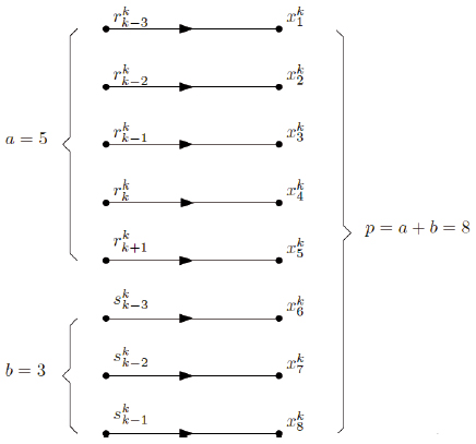
where a ∈ℤ⁺ indicates the number of components of the input vector containing past and future rainfall information represented by r, and b ∈ℤ⁺ represents the number of input vector terms containing past inflow records represented by s, with p=a+b. It means that if we are forecasting the streamflow for time instant k, rainfall terms composing the input patterns will consider the last a - 1accumulated B days rainfall lags, the expected accumulated B days rainfall for instant k, as well as the last b inflows recorded up to k - 1as input variables. For the next h steps ahead, forecasted inflows and rainfall will be necessary. Figure 3 shows a signal flow diagram for the mapping of time-series into input space, considering a=5 and b=3.

Figure 3
Signal flow diagram.

With the purpose of improving the explanatory power of the rainfall time series for each hydro plant, the FIS model uses as rainfall variable the accumulated precipitation of the last B days, where B is selected by maximizing the correlation coefficients between observed runoff and accumulated precipitation during those B days. Optimal B values for all the three inflow time series as well as correlation coefficient achieved are presented in Table 2.

Table 2
Optimal B values, correlation coefficients, and lags for buildinginput patterns considering rainfall and runoff information.

Plant	B	Correlation	a	b
NAV	6	0.73	4	3
BAR	5	0.74	5	3
BBO	4	0.76	5	1

Table 2 also shows the number of lags a and b considered as input variables for modeling each model. These numbers of lags were selected by maximizing the model performance for a multi-step ahead daily inflow forecasting task, with time horizon varying from one to twelve days ahead. As observed, in the case of runoff (b), the first three lags of NAV and BAR and the first one of BBO were considered as input variables. In the case of accumulated precipitation, thelags considered varied from 4 to 6 days.

After input-output patterns are built, data set is normalized to the unit interval and then split up in two subsets: a training data set and a testing data set. The training data set was composed by the first two years of historical data, whereas the testing data set was composed by the last one. Initial spreads for the SC algorithm (r ² _a ) was equal to 1.25.

5 ANALYSIS OF RESULTS

In this section, two components of the advanced queries module were utilized: statistical and graphical analysis. The first was employed to evaluate the performance of the hydrologic models using the following metrics: MAPE, RMSE, MAE, and E. The second component was used to facilitate the visual comparison between observed and predicted inflows.

The statistics are given for a forecasting horizon h varying from 1,…,12 months. Since FIS provides a different forecasted trajectory for each time instant, columns 2 to 13 present average errors of the last 353 predicted trajectories from one to twelve steps ahead.

Figure 4 shows the MAPE between observed and forecasted inflows for NAV, BAR, and BBO from 01/01/2007 to 12/31/2007, for one to up to twelve days ahead multi-step forecasting task. The worst performance in terms of MAPE was obtained by the BBO plant. The NAV plant presented the lowest MAPE. However, since this metric is a relative index, it is necessary to consider at least another absolute performance metric, as follows.

Figure 4
MAPE values for NAV, BAR, and BBO.

Table 3 shows the RMSE and MAE between observed and forecasted inflows for the same set of plants and the same time period, for h=1,…,12. Considering the RMSE, the BBO plant presents better results than both the NAV and the BAR from the third month on. Likewise, the BBO plant outperforms NAV and BAR from the fourth month onwards regarding MAE.It means that the BBO plant achieved, on average, better results than NAV and BAR for RMSE and MAE. The highest values are presented by the NAV plant, which is expected due to the inflow levels.

Table 3
RMSE and MAE values for NAV, BAR, and BBO.

Plant	Horizon (h) - months
	1	2	3	4	5	6	7	8	9	10	11	12
Root Mean Square Error (RMSE) - m3/s
NAV	4.40	7.34	9.44	10.81	11.70	12.29	12.67	12.94	13.10	13.21	13.27	13.31
BAR	3.67	5.76	7.18	8.06	8.60	8.92	9.04	9.04	9.01	8.96	8.92	8.87
BBO	5.06	6.20	7.00	7.55	7.94	8.13	8.19	8.19	8.18	8.16	8.14	8.13
Mean Absolute Error (MAE) - m3/s
NAV	36.09	60.77	81.89	98.06	110.28	119.91	126.86	132.08	135.77	138.63	140.80	142.29
BAR	37.57	55.75	69.85	80.16	87.25	91.96	94.94	96.71	97.93	98.94	99.73	100.39
BBO	51.40	62.07	70.26	76.27	80.67	83.72	85.85	87.44	88.73	89.74	90.57	91.29

The next performance metric is known as Mass Curve Coefficient (E). It is defined by Eq. (14):

(14)

where ȳ is the observed mean inflow. The first sum in the numerator denotes the total Square Error (SE) achieved - assuming as forecast inflow the historical mean for all k. The second sum represents the SE achieved by the evaluated model (FIS). Therefore, the closer E is to the unity, the better the model is, since the respective SE will be lower than the SE given by the mean.

Table 4 shows the E values, again, for the same set of plants and the same time period. Regarding explanatory power, the FIS presented a Mass Curve Coefficient (E) varying from 82% to 98% for NAV, 79% to 97% for BAR, and 79% to 93% for BBO.

Table 4
E values for NAV, BAR, and BBO.

Plant	Horizon (h) - months
	1	2	3	4	5	6	7	8	9	10	11	12
Mass Curve Coefficient (E)
NAV	0.98	0.95	0.92	0.89	0.88	0.86	0.85	0.84	0.84	0.83	0.83	0.82
BAR	0.97	0.93	0.89	0.86	0.84	0.82	0.81	0.81	0.80	0.80	0.80	0.79
BBO	0.93	0.90	0.87	0.85	0.83	0.82	0.81	0.81	0.80	0.80	0.80	0.79

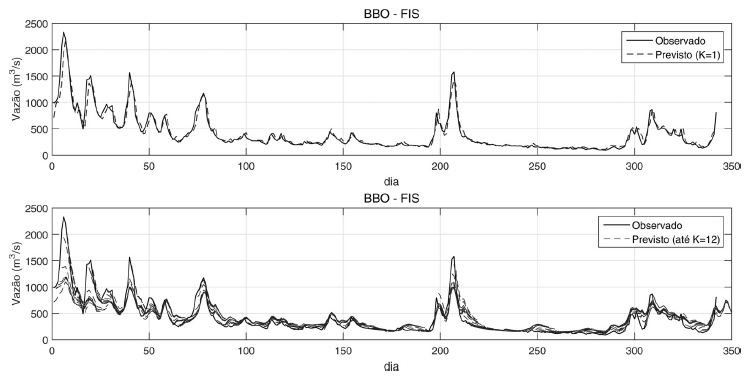
Forecast trajectories for one-step ahead and for one up to twelve-steps ahead are shown in Figures 5, 6, and 7, for NAV, BAR, and BBO, respectively. It is possible to realize that the difficulty in predicting inflows increases during humid periods. This occurs because the different trajectories obtained at the beginning of the year tend to be apart from the observed one with the increase of the lead time and especially before the peak flows.

Figure 5
One-step ahead and one up to twelve-step-ahead daily inflow forecasting for NAV plant.

Figure 6
One-step ahead and one up to twelve-step-ahead daily inflow forecasting for BAR plant.

Figure 7
One-step ahead and one up to twelve-step-ahead daily inflow forecasting for BBO plant.

These results can be compared with the output from other known forecasting methods. We have chosen two models: PREVIVAZ and MLRM.

PREVIVAZ analyzes the historical series of weekly inflows of each hydroelectric and selects, for each week, a model from several alternatives of stochastic modeling. These alternatives based on the time series models proposed by Box and Jenkins, more specifically, autoregressive models with or without moving mean component; AR and ARMA, respectively. These models are constructed as a function of past information in different time steps (lags). They may or may not to show periodic correlation structure. The temporal correlation structure of the series of weekly inflow is defined at intervals of different durations (weekly, monthly, quarterly and half-yearly). In addition, the parameters of these models are estimated using different methods (method of moments, regression). The definition of the modeling alternatives can be made from a prior processing (Box-Cox and/or logarithmic) of the series of weekly inflows (^{CEPEL, 2016}).

PREVIVAZ has been chosen because it is the current forecasting model used by ONS. According to (^{ONS, 2008}), in 2007, the mean percentage error in the inflow forecasting was of 30% for NAV, 33% for BAR, and 37% for BBO.

MLRM is a linear regression model with more than two explanatory variables. Therefore, it is a multiple linear regression model. MLRM models the relationship among the inflow to observed rainfalls (the previous five days) and observed inflows (the previous two days) by fitting a linear equation. It uses the least square method that minimizes the sum of the squares of residuals - vertical deviations from each data point to the line (^{Hidalgo et al., 2015}).

MLRM has been chosen because it is a very simple and fast technique that requires few variables. For the coefficients adjusted as described in (^{Hidalgo et al., 2015}), the mean percentage error for NAV, BAR, and BBO is around 12% with the best result for BAR and the worst result for NAV.

6 CONCLUSIONS AND FUTURE RESEARCH

This paper presented the evaluation of a TS-FIS model embedded in a tool developed to run inflow forecasting models and aid the analysis of their results. The model was adjusted for three Brazilian hydroelectric plants that belong to the interconnected power system of the country.

Different metrics were used to validate the model, i.e. MAPE, RMSE, MAE, and E. They showed satisfactory performance especially for short forecasting horizons. It was possible to realize that the performance of the model becomes degraded as the forecast horizon moves away from the actual time instant. This happens because the prediction errors of the previous steps feed into the input pattern for the next step ahead. However, given that the value of the mass curve coefficient varies from 79% to 98%, we can consider that the model presents an adequate performance due to its capability of explaining the hydrological process in at least 79%.

As future research the authors consider three suggestions. The first is the application of evolutionary algorithms to optimize model parameters. The fitness function of these algorithms may incorporate forecasting errors n-steps ahead.

The second suggestion consists of adjusting two forecasting models. One of them is adjusted for the humid period that shows higher variability of the inflows, and another one for the dry period where inflow behavior is more predictable.

As a third suggestion, it is also interesting to analyze the results from the combination of different models adjusted for the same goal. For example, one based on FIS and the other based on linear regression. Previous work in this area demonstrates that joining predictors may lead to a decrease in forecasting errors, especially in multiple-steps ahead prediction.

ACKNOWLEDGMENTS

This work was supported by FAPESP, Brazilian Agency dedicated to the development of science and technology (Process: 2011/09178-1); and by the AES Tietê company (Process: 37-P-17852-2010).

REFERENCES

• ¹
  AES-Tiete. 2016. AES-Tiete power generation company. Available from: Available from: http://www.aestiete.com.br/ Accessed on: 10/06/2016.
  » http://www.aestiete.com.br/
• ²
  ANNEL. 2007. New model of inflow forecasting with precipitation information for Itaipu. Electric Energy National Agency. Available from: Available from: http://www2.aneel.gov.br/aplicacoes/consulta_publica/documentos/NT_%20173-2007_Modelo_SMAP-MEL_Itaipu.pdf Accessed on: 09/09/2016.
  » http://www2.aneel.gov.br/aplicacoes/consulta_publica/documentos/NT_%20173-2007_Modelo_SMAP-MEL_Itaipu.pdf
• ³
  ANEEL 2008. Atlas of electric energy in Brazil (3rd edition). Electric Energy National Agency. Available from: Available from: www.aneel.gov.br Accessed on: 10/06/2016.
  » www.aneel.gov.br
• ⁴
  BOWDEN GJ, MAIER HR & DANDY GC. 2005. Input determination for neural network models in water resources applications (part 2). Case study: Forecasting salinity in a river. Journal of Hydrology, 301: 93-107.
• ⁵
  BRAVO JM, PAZ AR, COLLISCHONN W, UVO CB, PEDROLLO OC & CHOU SC. 2009. Incorporating forecasts of rainfall in two hydrologic models used for medium-range streamflow forecasting. Journal of Hydrologic Engineering, 14(5): 435-445.
• ⁶
  CEPEL 2016. Center for Energy Research. Available from: Available from: http://www.cepel.br/produtos/previvaz-modelos-computacionais-para-previsao-de-afluencias-diarias-semanais-e-mensais.htm Accessed on: 10/06/2016.
  » http://www.cepel.br/produtos/previvaz-modelos-computacionais-para-previsao-de-afluencias-diarias-semanais-e-mensais.htm
• ⁷
  CHIU S. 1994. A cluster estimation method with extension to fuzzy model identification. In: Proceedings of The IEEE International Conference on Fuzzy Systems, 2: 1240-1245.
• ⁸
  COULIBALY P, HACHÉ M, FORTIN V & BOBÉE B. 2005. Improving daily reservoir inflow forecasts with model combination. Journal of Hydrologic Engineering, 10(2): 91-99.
• ⁹
  D’ANGELO MFSV, PALHARES RM, TAKAHASHI RHC & LOSCHI RH. 2011. A fuzzy/Bayesian approach for the time series change point detection problem. Pesquisa Operacional, 31(2): 217-234.
• ¹⁰
  DAWSON C & WILBY R. 2001. Hydrological modelling using artificial neural networks. Progress in Physical Geography, 25(1): 80-108.
• ¹¹
  HIDALGO I, FONTANE D, ARABI M, LOPES J, ANDRADE J & RIBEIRO L. 2012. Evaluation of optimization algorithms to adjust efficiency curves for hydroelectric generating units. Journal of Energy Engineering, 138(4): 172-178.
• ¹²
  HIDALGO I, FONTANE D, LOPES J, ANDRADE J & DE ANGELIS A. 2014. Efficiency curves for hydroelectric generating units. Journal of Water Resources Planning and Management, 140(1): 86-91.
• ¹³
  HIDALGO I G, BARBOSA PSF, FRANCATO AL, LUNA I, CORREIA PB & PEDRO PSM. 2015. Management of Inflow Forecasting Studies. Water Practice & Technology, 10(2): 402-408.
• ¹⁴
  JACOBS R, JORDAN M, NOWLAN S & HINTON G. 1991. Adaptive mixture of local experts. Neural Computation, 3(1): 79-87.
• ¹⁵
  JIMOH RG, OLAGUNJU M, FOLORUNSO IO & ASIRIBO MA. 2013. Modeling rainfall prediction using fuzzy logic. International Journal of Innovative Research in Computer and Communication Engineering, 1(4): 929-936.
• ¹⁶
  LAZARO M, SANTAMARIAA I & PANTALEON C. 2003. A new EM-based training algorithm for RBF networks. Neural Networks, 16(1): 69-77.
• ¹⁷
  LOPES JEG, BRAGA BPF & CONEJO JGL. 1982. SMAP - A simplified hydrologic model. Applied modelling in catchment hydrology/ Ed. V.P. Singh. Water Resources Publication, Littleton, Colorado, USA, 167-176.
• ¹⁸
  LOPES J EG. 2007. Model for operation planning of hydrothermal systems for electrical energy production. Ph.D. thesis, University of São Paulo, Brazil (in Portuguese).
• ¹⁹
  LUNA I, SOARES S, LOPES JEG & BALLINI R. 2009. Verifying the use of evolving fuzzy systems for multi-step ahead daily inflow forecasting. 15th International Conference on Intelligent System Applications to Power Systems - ISAP, pp. 166. Doi: 10.1109/ISAP.2009.5352814.
  » https://doi.org/10.1109/ISAP.2009.5352814
• ²⁰
  LUNA I & BALLINI R. 2011. Top-down strategies based on adaptive fuzzy rule-based systems for daily time series forecasting. International Journal of Forecasting, 27(3): 708-724. Doi:10.1016/j.ijforecast.2010.09.006.
  » https://doi.org/10.1016/j.ijforecast.2010.09.006
• ²¹
  LUNA I, BALLINI R , SOARES S & FILHO DS. 2011. Fuzzy inference systems for synthetic monthly inflow time series generation. In P. published by Atlantis Press, (7th edition) conference of the European Society for Fuzzy Logic and Technology, pp. 1-7.
• ²²
  MELO B, MILIONI AZ & NASCIMENTO JÚNIOR CL. 2007. Daily and monthly sugar price forecasting using the mixture of local expert models. Pesquisa Operacional, 27(2): 235-246.
• ²³
  NAYAK P, SUDHEER K, RANGAN D & RAMASASTRI K. 2004. A neuro-fuzzy computing technique for modeling hydrological time series. Journal of Hydrology, 291: 52-66.
• ²⁴
  ONS. 2008. Annual evaluation report of inflow forecasting - 2007. Operator of the National Electric System. Available from: Available from: www.ons.org.br Accessed on: 10/05/2015.
  » www.ons.org.br
• ²⁵
  ONS. 2010. Inflow Forecasting. Operator of the National Electric System. Available from: Available from: www.ons.org.br Accessed on: 10/06/2016.
  » www.ons.org.br
• ²⁶
  SOMAR. 2016. Somar Meteorology. Available from: Available from: www.somarmeteorologia.com.br Accessed on: 10/06/2016.
  » www.somarmeteorologia.com.br
• ²⁷
  SOUSA FILHO FA & LALL U. Model of sazonal and interanual inflow forecasting. Revista Brasileira de Recursos Hídricos, 9(2): 61-74 (in Portuguese).
• ²⁸
  TAKAGI T & SUGENO M. 1985. Fuzzy identification of systems and its applications to modelingand control. IEEE Transactions on Systems, Man and Cybernetics, 15(1): 116-132.
• ²⁹
  WONG WK, XIA MIN & CHU WC. 2010. Adaptive neural network model for time-series forecasting. European Journal of Operational Research, 207(2): 807-816.
• ³⁰
  ZAMBELLI M, LUNA I & SOARES S. 2009. Long-term hydropower scheduling based on deterministic nonlinear optimization and annual inflow forecasting models. PowerTech, IEEE Bucharest, pp. 1-8.
• ³¹
  ZHANG J, CHENG C-T, LIAO S-L, WU X-Y & SHEN J-J. 2009. Daily reservoir inflow forecasting combining QPF into ANNs Model. Hydrology Earth System Sciences Discussions, 6: 121-150.

Publication Dates

• Publication in this collection
  Jan-Apr 2017

History

• Received
  28 June 2016
• Accepted
  16 Mar 2017