Topp–Leone odd log-logistic exponential distribution: Its improved estimators and applications

Abstract

In this paper, a new three-parameter lifetime model called the Topp–Leone odd log-logistic exponential distribution is proposed. Its density function can be expressed as a linear mixture of exponentiated exponential densities and can be reversed-J shaped, skewed to the left and to the right. Further, the hazard rate function of the new model can be monotone, unimodal, constant, J-shaped, constant-increasing-decreasing and decreasing-increasing-decreasing and bathtub-shaped. Our main focus is on estimation from a frequentist point of view, yet, some statistical and reliability characteristics for the proposed model are derived. We briefly describe different estimators namely, the maximum likelihood estimators, ordinary least-squares estimators, weighted least-squares estimators, percentile estimators, maximum product of spacings estimators, Cramér-von-Mises minimum distance estimators, Anderson-Darling estimators and right-tail Anderson-Darling estimators. Monte Carlo simulations are performed to compare the performance of the proposed methods of estimation for both small and large samples. We illustrate the performance of the proposed distribution by means of two real data sets and both the data sets show the new distribution is more appropriate as compared to some other well-known distributions.

Key words
Bathtub failure rate; exponential distribution; maximum likelihood; skewed data; simulation

1 - INTRODUCTION

Statisticians have been interested in defining new classes of univariate distributions by adding one or more shape parameters to a baseline model to generate new extended distributions that provide greater flexibility in modeling real data in many applied fields. The exponential (Ex) distribution has been extensively used for analysing lifetime data because it is analytically tractable and has a lack of memory property. However, its applicability is limited since it exhibits only a constant hazard rate and its density function is decreasing.

Recently, many authors have proposed many generalizations of the Ex distribution to improve its flexibility. For example, the exponentiated Ex (EEx) by Gupta & Kundu (2001), beta-Ex (BEx) by Jones (2004) and Nadarajah & Kotz (2006), beta generalized Ex(BGEx) by Barreto-Souza et al. (2010), transmuted generalized Ex (TGEx) by Khan et al. (2017), Harris extended Ex (HEEx) by Pinho et al. (2015), Kumaraswamy transmuted Ex (KTEx) by Afify et al. (2016), Marshall–Olkin Nadarajah–Haghighi (MONH) by Lemonte et al. (2016), modified-Ex by Rasekhi et al. (2017), alpha-power Ex (APEx) by Mahdavi & Kundu (2017), odd exponentiated half-logistic Ex by Afify et al. (2018), Marshall–Olkin logistic-Ex (MOLEx) by Mansoor et al. (2019), generalized odd log-logistic Ex by Afify et al. (2019), extended Weibull-Ex by Afify & Mohamed (2020), alpha-power exponentiated-Ex by Afify et al. (2020), and transmuted Burr-X Ex distributions by Al-Babtain et al. (2021).

Our aim in this paper is to define and study a new three-parameter lifetime model called Topp–Leone odd log-logistic exponential (TLOLLEx) distribution, which has several desirable properties. The CDF of the TLOLLEx distribution is given by

$$F(x;a,b,\lambda )={\{1-{[1-\frac{{[1-exp(-\lambda x)]}^a}{exp(-\lambda ax)+{[1-exp(-\lambda x)]}^a}]}^2\}}^b,$$(1)

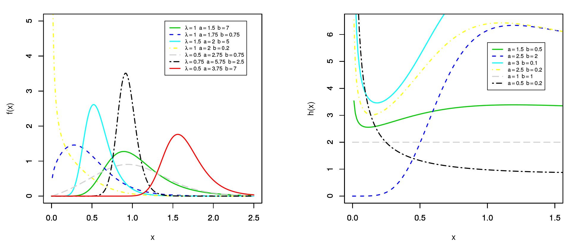
for all $x0$, $a0,b0$ and $\lambda 0$. The TLOLLEx distribution is an important model due to its flexibility in modeling all kinds of failure rate forms including monotone, bathtub, constant, upside-down bathtub, decreasing-increasing-decreasing and constant-increasing-decreasing (see Figure 1), which are common in reliability studies and lifetime data analysis. The above cited features make this distribution superior to other lifetime distributions which exhibit only monotonically increasing/decreasing or constant hazard rates. The TLOLLEx distribution can be viewed as a mixture of exponentiated exponential densities and the probability density function (PDF) of the TLOLLEx model can be reversed-J shaped, unimodal, symmetric, right-skewed and left-skewed. It may serve as a good alternative for fitting the skewed data in a variety of problems in different areas such as public health, environmental studies, biomedical studies, reliability and survival analysis. By means of two applications, we show that the TLOLLEx model provides better fits than at least ten other well-known extensions of the Ex distribution.

Figure 1
Left Panel: Plots of the TLOLLEx PDF for some selected values of the parameters. Right Panel: Plots of the TLOLLEx HRF for some selected values of the parameters.

Further, we are also motivated to show how different frequentist estimators of this distribution perform for different sample sizes and different parameter values and to develop a guideline for choosing the best estimation method, which we think would be of more interest to the applied statisticians. We consider the inferential procedures for estimating the parameters of TLOLLEx distribution - the maximum likelihood estimators (MLE), ordinary least-squares estimators (OLSE), weighted least-squares estimators (WLSE), maximum product of spacings estimators (MPSE), Cramer-von Mises minimum distance estimators (CVME), Anderson-Darling estimators (ADE) and right-tail Anderson-Darling estimators (RADE). The performance of these estimators are compared using extensive numerical simulations. Similar studies for other distributions have been carried out by several authors (see Louzada et al. 2016, Dey et al. 2017, Rodrigues et al. 2018, Nassar et al. 2018, and Nassar et al. 2020).

The rest of the article is outlined as follows. In Section 2, we define the TLOLLEx distribution and provide some plots for its HRF and PDF. In Section 3, we obtain some general mathematical properties of this distribution. In Section 4, eight different estimation methods of the unknown parameters are presented. In Section 5, we perform a simulation study to evaluate the performance of the aforementioned estimation methods. The potentiality of the TLOLLEx distribution is also illustrated by means of two real data sets in Section 6. Finally, in Section 7, we provide some conclusions.

2 - GENESIS

Recently, Brito et al. (2017) proposed a new class of distributions called the Topp–Leone odd log-logistic-G (TLOLL-G) family with two extra shape parameters. The cumulative distribution function (CDF) of the TLOLL-G family is defined by

$$F(x;a,b,𝛗)={\{1-{[1-\frac{G{(x;𝛗)}^a}{G{(x;𝛗)}^a+\overline{G}{(x;𝛗)}^a}]}^2\}}^b,$$(2)

where $G(x;𝛗)$ is a baseline CDF with a $p\times 1$ vector of unknown parameters $𝛗$, $a0$ and $b0$ . The corresponding PDF of (2) reduces to

$$\begin{array}{r}f(x;a,b,\phi )=\frac{2abg(x;\phi )G{(x;\phi )}^{a-1}\overline{G}{(x;\phi )}^{2a-1}}{{\{G{(x;\phi )}^a+\overline{G}{(x;\phi )}^a\}}^3}\\ \times {\{1-{[1-\frac{G{(x;\phi )}^a}{G{(x;\phi )}^a+\overline{G}{(x;\phi )}^a}]}^2\}}^{b-1},\end{array}$$(3)

where $g(x;𝛗)$ is a baseline PDF with a vector of parameters $𝛗$. If $X$ is a random variable (rv) having the PDF (3), we can write $X\sim$TLOLL-G($a,b,𝛗$).

The hazard rate function (HRF) of the TLOLL-G class is given by

$$\tau (x;a,b,\phi )=\frac{\frac{2abg(x;\phi )G{(x;\phi )}^{a-1}}{{\{G{(x;\phi )}^a+\overline{G}{(x;\phi )}^a\}}^3}{\{1-{[1-\frac{G{(x;\phi )}^a}{G{(x;\phi )}^a+\overline{G}{(x;\phi )}^a}]}^2\}}^{b-1}}{\overline{G}{(x;\phi )}^{1-2a}(1-{\{1-{[1-\frac{G{(x;\phi )}^a}{G{(x;\phi )}^a+\overline{G}{(x;\phi )}^a}]}^2\}}^b)}.$$

Now, by considering the CDF and PDF of the Ex distribution, which are given by

$$G(x;\lambda )=1-exp(-\lambda x)\mathrm{\text{and}}g(x;\lambda )=\lambda exp(-\lambda x),$$(4)

respectively, where $\lambda$ is a positive scale parameter. Then, the PDF corresponding to (3) follows as

$$\begin{array}{r}f(x;a,b,\lambda )=\frac{2ab\lambda {[1-\exp (-\lambda x)]}^{a-1}\exp (-2\lambda ax)}{{\{\exp (-\lambda ax)+{[1-\exp (-\lambda x)]}^a\}}^3}\\ \times {(1-{\{1-\frac{{[1-\exp (-\lambda x)]}^a}{\exp (-\lambda ax)+{[1-\exp (-\lambda x)]}^a}\}}^2)}^{b-1},\end{array}$$(5)

where $\lambda 0$ is a scale parameter and $a0$ and $b0$ are shape parameters. The rv $X$ having the PDF (5) is denoted by $X\sim$TLOLLEx($\lambda ,a,b$).

Figure 1 shows some possible shapes of the HRF and PDF of the TLOLLEx distribution for some selected values of the model parameters. The HRF of the TLOLLEx model has the advantage of being capable of modeling various shapes including constant, increasing, decreasing, bathtub, unimodal, decreasing-increasing-decreasing and constant-increasing-decreasing. Plots of the PDF of the TLOLLEx distribution show that it can be reversed-J shaped, right-skewed and left-skewed. The TLOLLEx distribution has an advantage over Weibull, gamma and exponentiated exponential distributions as these distributions cannot model phenomenon showing non-monotone failure rates (bathtub and unimodal) and therefore TLOLLEx distribution seems to be more flexible for analyzing survival data.

3 - SOME PROPERTIES

Remark 1: The quantile function (QF) of $X$, $x=Q\left(u\right)=F^{-1}\left(u\right)$, follows as

$$Q\left(u\right)=\frac{-1}{\lambda }log\{1-\frac{{[{(1-u^{1/b})}^{-1/2}-1]}^{1/a}}{1+{[{(1-u^{1/b})}^{-1/2}-1]}^{1/a}}\}.$$

Hence, the TLOLLEx distribution can be easily simulated as follows: if $U$ has a uniform $U(0,1)$ distribution, then $X$ $=Q\left(U\right)$ has the PDF (5).

Remark 2: The PDF of the TLOLLEx distribution can be expressed as a mixture of exponentiated Ex PDFs (see Brito et al. 2017)

$$f\left(x\right)=\sum _{k=0}^{\infty }{d}_{k+1}(k+1)\lambda exp(-\lambda x){[1-exp(-\lambda x)]}^k,$$

where $d_{k+1}={\sum }_{i=0}^{\infty }{\sum }_{j=0}^{2i}{(-1)}^{i+j}\left(\genfrac{}{}{0ex}{}{b}{i}\right)\left(\genfrac{}{}{0ex}{}{2i}{j}\right)c_{k,j}.$ More details can be explored in Brito et al. (2017).

Using the generalized binomial expansion, the TLOLLEx PDF can be expressed as a linear combination of Ex densities, namely

$$f\left(x\right)=\sum _{m=0}^{\infty }{b}_m{g}_{m+1}(x;(m+1)\lambda ),$$(6)

where $b_m={\sum }_{k=0}^{\infty }\frac{{(-1)}^m}{m+1}\left(\genfrac{}{}{0ex}{}{k}{m}\right)d_{k+1}$ and $g_{m+1}(x;(m+1)\lambda )$ is the Ex density with scale parameter $(m+1)\lambda$.

Based on Remark 2, several mathematical properties of the TLOLLEx distribution can be obtained from those of the Ex distributions.

Let $Z$ be a rv having the Ex distribution (4). Then, the $n$th ordinary and incomplete moments of $Z$ are given, respectively, by

$${\mu }_{n,Z}^{\mathrm{\prime }}={\lambda }^{-n}\mathrm{\Gamma }(n+1)\text{and}{\varphi }_{n,Z}\left(t\right)={\lambda }^{-n}\gamma (n+1,\lambda t),$$

where $\Gamma (\cdot )$ and $\gamma (\cdot ,\cdot )$ are the complete and lower incomplete gamma functions, respectively.

Then, the $r$th ordinary moment of $X$ follows from (6) as

$${\mu }_r^{\prime }=\sum _{m=0}^{\infty }{b}_m{\left[(m+1)\lambda \right]}^{-r}\Gamma (r+1).$$

Based on (6), the $r$th incomplete moment of $X$ can be written as

$${\varphi }_r\left(t\right)=\sum _{m=0}^{\infty }{b}_m{\left[(m+1)\lambda \right]}^{-r}\gamma (r+1,(m+1)\lambda t).$$(7)

The moment generating function of the TLOLLEx distribution follows from (6) as

$$M_X\left(t\right)=\sum _{m=0}^{\infty }{b}_m\frac{(m+1)\lambda }{(m+1)\lambda -t}.$$

The values of mean, variance, skewness and kurtosis of TLOLLEx distribution are reported in Table I The values of these measures are computed numerically for $\lambda =1$ and some selected values of $a$ and $b$ using the R software (version 3.6) (R Core Team 2019). The numerical values show that the skewness of the TLOLLEx distribution can range in the interval $(-0.09,4.02)$ and decreases as $a$ and $b$ increases. The spread of the kurtosis is much larger, ranging from $3.0$ to $24.5$ and shows the similar behavior as skewness.

Table I
Mean, variance, skewness and kurtosis of the TLOLLEx distribution with $$\lambda =1$$ and different values of $a$ and $b$.

$a$	$b$	Mean	Variance	Skewness	Kurtosis
0.5	0.5	0.3140	0.5292	4.0221	24.5365
	1.5	0.7875	1.1425	2.3394	10.2340
	2.5	1.1396	1.4710	1.8382	7.4972
	4	1.5385	1.7318	1.4987	6.0702
	10	2.4690	1.9991	1.1164	4.9522
1.5	0.5	0.3447	0.1079	1.7054	7.3962
	1.5	0.6238	0.1333	1.2898	5.9634
	2.5	0.7675	0.1376	1.2380	5.8615
	4	0.9024	0.1399	1.2257	5.8562
	10	1.1687	0.1433	1.2328	5.8926
2.5	0.5	0.4158	0.0618	0.7678	3.8720
	1.5	0.6318	0.0514	0.7704	4.4737
	2.5	0.7248	0.0470	0.8809	4.8552
	4	0.8060	0.0442	0.9824	5.1794
	10	0.9565	0.0415	1.1327	5.6726
5	0.5	0.5168	0.0268	-0.0850	3.0036
	1.5	0.6541	0.0139	0.2950	3.7368
	2.5	0.7037	0.0113	0.5305	4.0772
	4	0.7444	0.0098	0.7097	4.4233
	10	0.8157	0.0083	0.9542	5.0511
7.5	0.5	0.9565	0.0415	1.1327	5.6726
	1.5	0.6652	0.0064	0.1251	3.6481
	2.5	0.6989	0.0049	0.4015	3.8669
	4	0.7261	0.0041	0.6027	4.1596
	10	0.7727	0.0034	0.8708	4.7555
20	0.5	0.7220	0.0004	0.7515	4.3566
	1.5	0.6817	0.0009	-0.0905	3.6799
	2.5	0.6947	0.0006	0.2353	3.6684
	4	0.7049	0.0005	0.4604	3.8551
	10	0.7220	0.0004	0.7515	4.3566

The Mean residual life (MRL) (also called life expectancy at age $t$, $t0$) is defined by

$$m_X\left(t\right)=[1-{\varphi }_1\left(t\right)]/S\left(t\right)-t,$$(8)

where $S\left(t\right)$ is the survival function of $X$. ${\varphi }_1\left(t\right)$ is the first incomplete moment of $X$ that follows from (7) with $r=1$ as

$${\varphi }_1\left(t\right)=\sum _{m=0}^{\infty }{b}_m\frac{\gamma (2,(m+1)\lambda t)}{(m+1)\lambda }.$$(9)

By substituting (9) in equation (8), we obtain the MRL of $X$ as

$$m_X\left(t\right)=\frac{1}{S\left(t\right)}\sum _{m=0}^{\infty }{b}_m\frac{\gamma (2,(m+1)\lambda t)}{(m+1)\lambda }-t.$$

The mean inactivity time (MIT) is defined (for $t0$) by

$$m_X^{\prime }\left(t\right)=t-\left[{\varphi }_1\left(t\right)/F\left(t\right)\right].$$(10)

By inserting (9) in equation (10), the MIT of $X$ becomes

$$m_X^{\prime }\left(t\right)=t-\frac{1}{F\left(t\right)}\sum _{m=0}^{\infty }{b}_m\frac{\gamma (2,(m+1)\lambda t)}{(m+1)\lambda }.$$

4 - PARAMETER ESTIMATION

In this section, we estimate the unknown parameters of the TLOLLEx distribution using eight frequentist estimators. These estimators are: the maximum likelihood estimators, least squares and weighted least-squares estimators, percentile based estimators, the maximum product of spacing estimators, Cramér–von Mises estimators, Anderson–Darling and Right-tail Anderson–Darling estimators.

4.1 - Maximum likelihood estimators

In this subsection, we consider the maximum likelihood method to estimate the unknown parameters of the TLOLLEx model from complete samples. Let $x_1,\dots ,x_n$ be a random sample of size $n$ from this distribution with parameter vector $j={(a,b,\lambda )}^{⊺}$. Then, the log-likelihood function for $j$ reduces to

$$\begin{array}{ccc}\hfill \ell & =\hfill & \hfill nlog2+nloga+nlogb+nlog\lambda +(a-1)\sum _{i=1}^{n}log[1-k_i]\\ \hfill & \hfill & \hfill -2\lambda a\sum _{i=1}^n{x}_i-3\sum _{i=1}^{n}log[k_i^a+{(1-k_i)}^a]\\ \hfill & \hfill & \hfill +(b-1)\sum _{i=1}^{n}log\{1-{[1-\frac{{(1-k_i)}^a}{k_i^a+{(1-k_i)}^a}]}^2\},\end{array}$$

where $k_i=exp(-\lambda x_i)$. The MLE of the unknown parameters $a$, $b$ and $\lambda$ of the TLOLLEx distribution can be obtained by maximizing the above equation. This can be done by using different programs namely R (optim function), SAS (PROC NLMIXED), or by solving the nonlinear likelihood equations obtained by differentiating $\ell$.

The components of the score vector, $$\mathbf{U}\left(\mathbf{j}\right)=\frac{\mathrm{\partial }\ell }{\mathrm{\partial }\mathbf{j}}={(\frac{\mathrm{\partial }\ell }{\mathrm{\partial }\lambda },\frac{\mathrm{\partial }\ell }{\mathrm{\partial }a},\frac{\mathrm{\partial }\ell }{\mathrm{\partial }b})}^{⊺}$$ , are given by

$$\begin{array}{r}\frac{\mathrm{\partial }\ell }{\mathrm{\partial }\lambda }=\frac{n}{\lambda }-2a\sum _{i=1}^n{x}_i+(a-1)\sum _{i=1}^n\frac{x_i{k}_i}{1-k_i}+3\sum _{i=1}^n\frac{a{x}_i{k}_i^a-z_i}{k_i^a+{(1-k_i)}^a}\\ -2(b-1)\sum _{i=1}^n\frac{{(1-k_i)}^a(z_i-a{x}_i{k}_i^a)-z_i[k_i^a+{(1-k_i)}^a]}{2k_i^a{(1-k_i)}^a+3{(1-k_i)}^{2a}+k_i^{-a}{(1-k_i)}^{3a}},\end{array}$$

$$\begin{array}{ccc}\hfill \frac{\partial \ell }{\partial a}& =\hfill & \hfill \frac{n}{a}-2\lambda \sum _{i=1}^n{x}_i+\sum _{i=1}^{n}log(1-k_i)-3\sum _{i=1}^n\frac{s_i}{k_i^a+{(1-k_i)}^a}\\ \hfill & \hfill & \hfill -2(b-1)\sum _{i=1}^n\frac{{(1-k_i)}^a{s}_i-{(1-k_i)}^a[k_i^a+{(1-k_i)}^a]log(1-k_i)}{2k_i^a{(1-k_i)}^a+3{(1-k_i)}^{2a}+k_i^{-a}{(1-k_i)}^{3a}}\end{array}$$

and

$$\frac{\partial \ell }{\partial b}=\frac{n}{b}+\sum _{i=1}^{n}log\{1-{[1-\frac{{(1-k_i)}^a}{k_i^a+{(1-k_i)}^a}]}^2\},$$

where $z_i=a{x}_{i}exp(-\lambda x_i){[1-exp(-\lambda x_i)]}^{a-1}$ and $s_i=k_i^{a}log{k}_i+{(1-k_i)}^a$ $log(1-k_i).$

Newton-Rapshon method can be used to find the solution of the nonlinear system of equations.

For simplicity, from $\partial \ell /\partial b=0$ for fixed $\lambda$ and $a$, we can obtain $\hat{b}(\lambda ,a)$ as

$$\begin{array}{c}\hfill \hat{b}(\lambda ,a)=-\frac{n}{\sum _{i=1}^{n}log\{1-{[1-\frac{{(1-k_i)}^a}{k_i^a+{(1-k_i)}^a}]}^2\}}\end{array}$$(11)

The MLE of $a$ and $\lambda$ are denoted by $\hat{a}$ and $\hat{\lambda }$, respectively. These estimates can be obtained by numerically by solving the following non-linear equations

$$\begin{array}{r}\frac{\mathrm{\partial }\ell }{\mathrm{\partial }\lambda }=\frac{n}{\lambda }-2a\sum _{i=1}^n{x}_i+(a-1)\sum _{i=1}^n\frac{x_i{k}_i}{1-k_i}+3\sum _{i=1}^n\frac{a{x}_i{k}_i^a-z_i}{k_i^a+{(1-k_i)}^a}\\ -2(\hat{b}(\lambda ,a)-1)\sum _{i=1}^n\frac{{(1-k_i)}^a(z_i-a{x}_i{k}_i^a)-z_i[k_i^a+{(1-k_i)}^a]}{2k_i^a{(1-k_i)}^a+3{(1-k_i)}^{2a}+k_i^{-a}{(1-k_i)}^{3a}}=0,\end{array}$$

and

$$\begin{array}{r}\frac{\mathrm{\partial }\ell }{\mathrm{\partial }a}=\frac{n}{a}-2\lambda \sum _{i=1}^n{x}_i+\sum _{i=1}^n\log (1-k_i)-3\sum _{i=1}^n\frac{s_i}{k_i^a+{(1-k_i)}^a}\\ -2(\hat{b}(\lambda ,a)-1)\sum _{i=1}^n\frac{{(1-k_i)}^a{s}_i-{(1-k_i)}^a[k_i^a+{(1-k_i)}^a]\log (1-k_i)}{2k_i^a{(1-k_i)}^a+3{(1-k_i)}^{2a}+k_i^{-a}{(1-k_i)}^{3a}}\\ =0.\end{array}$$(12)

Using iterative techniques to compute $\hat{\lambda }$ and $\hat{a}$ from (12), the MLE of $b$, $\hat{b}(\lambda ,a)$ can be computed from (11) as $\hat{b}(\hat{\lambda },\hat{a})$. For the TLOLLEx distribution, all the second order derivatives exist.

To avoid the initial values problem to estimate the parameters, we suggest using the initial value for the parameter $\lambda$ as ${\lambda }_0=1/\bar{X}$, because this parameter comes from the Ex distribution. For the initial value of the parameter $a$, we have used the grid initial values search procedure on the interval $(0,max\{X_1,X_2,...,X_n\}]$. We ran this procedure over possible values of the parameter $a$, to get $a_0$, and the initial value of the parameter $b$ is $b_0=b({\lambda }_0,a_0)$.

For interval estimation of the model parameters, we require $3\times 3$ observed information matrix $J\left(\vartheta \right)=\{J_{rs}\}$ for $r,s=a,b,\lambda$. Under standard regularity conditions, the multivariate normal $N_3(0,J{\left(\hat{\vartheta }\right)}^{-1})$ distribution can be used to construct approximate confidence intervals for the parameters. Here, $$J(\hat{\vartheta })$$ is the total observed information matrix evaluated at $$\hat{\vartheta }$$. An $100(1-\alpha )\%$ asymptotic confidence interval for each parameter ${\vartheta }_r$ is given by

$$AC{I}_r=({\hat{\vartheta }}_r-z_{\frac{\alpha }{2}}s.e.\left(\hat{\vartheta }\right),{\hat{\vartheta }}_r+z_{\frac{\alpha }{2}}s.e.\left(\hat{\vartheta }\right))$$

where $z_{{}_{\alpha /2}}$ is the upper ${\left(\alpha /2\right)}^{th}$ quantile of the standard normal distribution, and $s.e.\left(\hat{\vartheta }\right)$ is the standard error of the estimated parameter $\vartheta$ and it is given by $s.e.\left(\hat{\vartheta }\right)=\sqrt{J_{rr}\left(\hat{\vartheta }\right)}$ for $r=a,b,\lambda$.

4.2 - Ordinary and weighted least-square estimators

Let $x_{\left(1\right)},x_{\left(2\right)},\cdots ,x_{\left(n\right)}$ be the order statistics of the random sample of size $n$ from $F(𝐱;a,b,\lambda )$. The OLSE (see Swain et al. (1988)) ${\hat{a}}_{LSE}$, $${\hat{b}}_{LSE}$$ and ${\hat{\lambda }}_{LSE}$ can be obtained by minimizing the following function

$$V(a,b,\lambda )=\sum _{i=1}^n{[F(x_{\left(i\right)}|a,b,\lambda )-\frac{i}{n+1}]}^2$$

with respect to $a,b$ and $\lambda$ or equivalently solving the following non-linear equation

$$\sum _{i=1}^n[F(x_{\left(i\right)}|a,b,\lambda )-\frac{i}{n+1}]{\Delta }_s(x_{\left(i\right)}|a,b,\lambda )=0,s=1,2,3,$$

where

$$\begin{array}{r}{\mathrm{\Delta }}_1(x_{(i)}|a,b,\lambda )=\frac{\mathrm{\partial }}{\mathrm{\partial }a}F(x_{(i)}|a,b,\lambda ),{\mathrm{\Delta }}_2(x_{(i)}|a,b,\lambda )=\frac{\mathrm{\partial }}{\mathrm{\partial }b}F(x_{(i)}|a,b,\lambda )\\ \text{and }{\mathrm{\Delta }}_3(x_{(i)}|a,b,\lambda )=\frac{\mathrm{\partial }}{\mathrm{\partial }\lambda }F(x_{(i)}|a,b,\lambda )\end{array}$$(13)

Note that the solution of ${\Delta }_s$ for $s=1,2,3$ can be obtained numerically.

The WLSE (Swain et al. (1988)), ${\hat{a}}_{WLSE}$, ${\hat{b}}_{WLSE}$ and ${\hat{\lambda }}_{WLSE}$, can be obtained by minimizing the following equation

$$W(a,b,\lambda )=\sum _{i=1}^n\frac{{(n+1)}^2(n+2)}{i(n-i+1)}{[F(x_{\left(i\right)}|a,b,\lambda )-\frac{i}{n+1}]}^2.$$

with respect to $a,b$ and $\lambda$ or the WLSE can also be obtained by solving the following non-linear equation

$$\sum _{i=1}^n\frac{{(n+1)}^2(n+2)}{i(n-i+1)}[F(x_{\left(i\right)}|a,b,\lambda )-\frac{i}{n+1}]{\Delta }_s(x_{\left(i\right)}|a,b,\lambda )=0,s=1,2,3,$$

where ${\Delta }_1(\cdot |a,b,\lambda )$, ${\Delta }_2(\cdot |a,b,\lambda )$ and ${\Delta }_3(\cdot |a,b,\lambda )$ are provided in (13).

4.3 - Percentile based estimation

Kao (1958) proposed the PCE. Let $u_i=i/(n+1)$ be an unbiased estimator of $F(x_{\left(i\right)}|a,b,\lambda )$. Then, the PCE of the parameters of TLOLLEx distribution can be obtained by minimizing the following function

$$P(a,b,\lambda )=\sum _{i=1}^n{(x_{\left(i\right)}-\frac{-1}{\lambda }log\{1-\frac{{[{(1-u_i^{1/b})}^{-1/2}-1]}^{1/a}}{1+{[{(1-u_i^{1/b})}^{-1/2}-1]}^{1/a}}\})}^2,$$

with respect to $a,b$ and $\lambda$.

4.4 - Method of maximum product of spacing

Cheng Amin (1983) are proposed independently the maximum product of spacings (MPSE) method, as an approximation to the Kullback-Leibler information measure and can be used as an alternative to the MLE method.

Let $D_i(a,b,\lambda )=F(x_{\left(i\right)}|a,b,\lambda )-F(x_{(i-1)}|a,b,\lambda )$, for $i=1,2,\dots ,n+1,$ be the uniform spacings of a random sample from the TLOLLEx distribution, where $F(x_{\left(0\right)}|a,b,\lambda )=0$, $F(x_{(n+1)}|a,b,\lambda )=1$ and ${\sum }_{i=1}^{n+1}{D}_i(a,b,\lambda )=1$. The MPSE ${\hat{a}}_{MPSE}$, ${\hat{b}}_{MPSE}$ and ${\hat{\lambda }}_{MPSE}$ can be obtained by maximizing the geometric mean of the spacing

$$G(a,b,\lambda )={\left[\prod _{i=1}^{n+1}{D}_i(a,b,\lambda )\right]}^{\frac{1}{n+1}}$$(14)

with respect to $a$, $b$ and $\lambda$, or, equivalently, by maximizing the logarithm of the geometric mean of spacing

$$H(a,b,\lambda )=\frac{1}{n+1}\sum _{i=1}^{n+1}log{D}_i(a,b,\lambda ).$$

The MPSE, ${\hat{a}}_{MPSE}$, ${\hat{b}}_{MPSE}$ and ${\hat{\lambda }}_{MPSE}$, of the TLOLLEx parameters can be obtained by solving the nonlinear equation defined by

$$\frac{1}{n+1}\sum _{i=1}^{n+1}\frac{1}{D_i(a,b,\lambda )}[{\Delta }_s(x_{\left(i\right)}|a,b,\lambda )-{\Delta }_s(x_{(i-1)}|a,b,\lambda )]=0,s=1,2,3,$$

where ${\Delta }_1(\cdot |a,b,\lambda )$, ${\Delta }_2(\cdot |a,b,\lambda )$ and ${\Delta }_3(\cdot |a,b,\lambda )$ are defined in (13).

4.5 - The Cramér-von Mises minimum distance estimators

MacDonald (1971) showed empirically that the CVME, as a type of minimum distance estimators (also called maximum goodness-of-fit estimators), have less bias than the other minimum distance estimators.

The CVME are obtained based on the difference between the estimates of the cumulative distribution function and the empirical distribution function.

The CVME of the TLOLLEx parameters are obtained by minimizing

$$C(a,b,\lambda )=\frac{1}{12n}+\sum _{i=1}^n{[F(x_{\left(i\right)}|a,b,\lambda )-\frac{2i-1}{2n}]}^2,$$

with respect to $a,b$ and $\lambda$. Also, the CVME can be obtained by solving the non-linear equation

$$\sum _{i=1}^n[F(x_{\left(i\right)}|a,b,\lambda )-\frac{2i-1}{2n}]{\Delta }_s(x_{\left(i\right)}|a,b,\lambda )=0,s=1,2,3,$$

where ${\Delta }_1(\cdot |a,b,\lambda )$, ${\Delta }_2(\cdot |a,b,\lambda )$ and ${\Delta }_3(\cdot |a,b,\lambda )$ are provided in (13).

4.6 - The Anderson-Darling and right-tail Anderson-Darling estimators

The Anderson-Darling statistic that is also known as the Anderson-Darling estimator is another type of minimum distance estimators. The ADE of the parameters of the TLOLLEx model are obtained by minimizing

$$A(a,b,\lambda )=-n-\frac{1}{n}\sum _{i=1}^n(2i-1)[logF(x_{\left(i\right)}|a,b,\lambda )+logS(x_{\left(i\right)}|a,b,\lambda )],$$

with respect to $a,b$ and $\lambda$. These ADE can also be obtained by solving the non-linear equation

$$\sum _{i=1}^n(2i-1)[\frac{{\mathrm{\Delta }}_s(x_{(i)}|a,b,\lambda )}{F(x_{(i)}|a,b,\lambda )}-\frac{{\mathrm{\Delta }}_j(x_{(n+1-i)}|a,b,\lambda )}{S(x_{(n+1-i)}|a,b,\lambda )}]=0,s=1,2,3.$$

The right-tail RADE of the TLOLLEx parameters are obtained by minimizing

$$R(a,b,\lambda )=\frac{n}{2}-2\sum _{i=1}^{n}F(x_{i:n}|a,b,\lambda )-\frac{1}{n}\sum _{i=1}^n(2i-1)logS(x_{n+1-i:n}|a,b,\lambda ),$$

with respect to $a,b$ and $\lambda$. The RADE can also be obtained by solving the non-linear equation

$$-2\sum _{i=1}^n{\Delta }_s(x_{i:n}|a,b,\lambda )+\frac{1}{n}\sum _{i=1}^n(2i-1)\frac{{\Delta }_s(x_{{}_{n+1-i:n}}|a,b,\lambda )}{S(x_{n+1-i:n}|a,b,\lambda )}=0,s=1,2,3.$$

where ${\Delta }_1(\cdot |a,b,\lambda )$, ${\Delta }_2(\cdot |a,b,\lambda )$ and ${\Delta }_3(\cdot |a,b,\lambda )$ are defined in equation (13).

5 - SIMULATION STUDY

In this section, we have carried out an extensive simulation study to compare the performance of the frequentist estimators discussed in the previous sections. The methods are compared for sample sizes $n=\{30,80,100,200,350\}$ with parameter values $a=(0.8,2.5),b=(1.2,6.0)$ and $\lambda =(1.5,5.0)$. We generate $N=5,000$ pseudo-random samples from TLOLLEx distribution using the inverse transform method. The following procedures are adopted to generate pseudo-random samples from TLOLLEx distribution.

• Generate pseudo-random values from the TLOLLEx distribution with size $n$.

• Using the obtained samples in step 1, calculate $\hat{a}$, $\hat{b}$ and $\hat{\lambda }$ via 1-WLSE, 2-OLSE, 3-MLE, 4-MPSE, 5-CVME, 6-ADE, 7-RADE, 8-PCE.

• Repeat the steps $1$ and $2$, $N$ times.

For each estimate, we calculate absolute bias, mean-squared error and mean relative error. These measures are obtained by using the following formulae: Average of absolute biases ($\left|Bias\left(\widehat{𝛉}\right)\right|$), $\left|Bias\left(\widehat{𝛉}\right)\right|=$ $\frac{1}{N}{\sum }_{i=1}^N|\widehat{𝛉}-𝛉|$, the average of mean squared error (MSEs), $MSEs=\frac{1}{N}{\sum }_{i=1}^N{(\widehat{𝛉}-𝛉)}^2$, and average of mean relative error (MREs), $MREs=\frac{1}{N}{\sum }_{i=1}^N|\widehat{𝛉}-𝛉|/𝛉$.

The performance of the considered estimators is evaluated in terms of absolute bias, mean-squared error and mean relative error. Considering this approach, the most efficient estimation method will be the one whose MRE value is closer to one and bias closer to zero. All simulations are done in R software (version 3.6) (R Core Team 2019).

In Tables II-IV we report the values of $\left|Bias\left(\widehat{𝛉}\right)\right|$, $MSEs$ and $MREs$ of the WLSE, OLSE, MLE, MPSE, CVME, ADE, RADE and PCE. Furthermore, a superscript indicates the rank of each of the estimators among all the estimators for that metric and the $\sum Ranks$, which is the partial sum of the ranks for each column in a certain sample size. Table VII shows the the partial and overall rank of the estimators. From Tables II-VII, we observe that:

• Most of the estimators reveal the property of consistency, i.e., the MSEs and MREs decreases as sample size increases, for all parameter combinations.

• Only the estimators MPSE and RADE are not consistent. They fail in finding the parameter estimates for a significant number of samples for all parameter combinations. So, these estimators are not recommended for the estimation of the TLOLLEx parameters.

• From Table VII, and for the parameter combinations, we can conclude that the MLE method outperforms all the other methods of estimation (overall score of 27). Therefore, depends on our study, we can consider that the MLE method is the optimal method to estimate the TLOLLEx parameters.

Table II
Simulation results for $𝛉={(a=0.8,b=6,\lambda =5)}^{⊺}$.

$n$	Est.	Est. Par.	WLSE	OLSE	MLE	MPSE	CVME	ADE	RADE	PCE
30	$\left|BIAS\right|$	$\hat{a}$	${0.43508}^6$	${0.10409}^2$	${0.10341}^1$	${2.8922}^8$	${0.33747}^4$	${0.36851}^5$	${0.69795}^7$	${0.27961}^3$
		$\hat{b}$	${3.86073}^7$	${0.92883}^2$	${0.89696}^1$	${3018.95274}^8$	${2.68968}^4$	${3.72972}^6$	${2.61118}^3$	${3.41521}^5$
		$\hat{\lambda }$	${8.08922}^6$	${0.10938}^2$	${0.10834}^1$	${241.54073}^8$	${5.03769}^4$	${6.35647}^5$	${48.29126}^7$	${4.29398}^3$
	$MSE$	$\hat{a}$	${0.60483}^7$	${0.01898}^2$	${0.01856}^1$	${28.51351}^8$	${0.52376}^6$	${0.31541}^4$	${0.50161}^5$	${0.15596}^3$
		$\hat{b}$	${24.14124}^6$	${1.48634}^2$	${1.38744}^1$	${19320316.43015}^8$	${16.35598}^4$	${24.50634}^7$	${7.05568}^3$	${18.46519}^5$
		$\hat{\lambda }$	${374.63511}^6$	${0.02506}^2$	${0.02411}^1$	${493093.06823}^8$	${140.27232}^4$	${243.02016}^5$	${3054.18764}^7$	${59.97591}^3$
	$MRE$	$\hat{a}$	${0.54385}^6$	${0.13012}^2$	${0.12926}^1$	${3.61525}^8$	${0.42184}^4$	${0.46063}^5$	${0.87244}^7$	${0.34952}^3$
		$\hat{b}$	${0.64345}^7$	${0.15480}^2$	${0.14949}^1$	${503.15879}^8$	${0.44828}^4$	${0.62162}^6$	${0.4352}^3$	${0.5692}^5$
		$\hat{\lambda }$	${1.61784}^6$	${0.02188}^2$	${0.02167}^1$	${48.30815}^8$	${1.00754}^4$	${1.27129}^5$	${9.65825}^7$	${0.8588}^3$
	$\sum$ Ranks		${57}^7$	${18}^2$	$9^1$	${72}^8$	${38}^4$	${48}^5$	${49}^6$	${33}^3$
80	$\left|BIAS\right|$	$\hat{a}$	${0.29306}^6$	${0.05847}^1$	${0.05938}^2$	${2.2639}^8$	${0.25398}^3$	${0.27124}^4$	${0.7478}^7$	${0.27262}^5$
		$\hat{b}$	${3.52071}^6$	${0.55506}^2$	${0.54882}^1$	${2016.96826}^8$	${3.06575}^4$	${3.46029}^5$	${2.51052}^3$	${3.53968}^7$
		$\hat{\lambda }$	${3.88719}^5$	${0.05833}^1$	${0.05916}^2$	${126.2829}^8$	${4.13892}^6$	${3.69441}^4$	${58.28086}^7$	${3.35589}^3$
	$MSE$	$\hat{a}$	${0.14794}^6$	${0.00562}^1$	${0.0058}^2$	${11.20443}^8$	${0.12023}^5$	${0.11575}^4$	${0.55978}^7$	${0.09614}^3$
		$\hat{b}$	${20.08317}^6$	${0.50599}^2$	${0.48506}^1$	${12758597.38963}^8$	${18.91885}^5$	${20.34719}^7$	${6.3579}^3$	${18.12801}^4$
		$\hat{\lambda }$	${57.04164}^5$	${0.00629}^1$	${0.0065}^2$	${240155.50936}^8$	${73.79332}^6$	${50.45261}^4$	${3678.59546}^7$	${29.14491}^3$
	$MRE$	$\hat{a}$	${0.36633}^6$	${0.07309}^1$	${0.07422}^2$	${2.82987}^8$	${0.31747}^3$	${0.33905}^4$	${0.93475}^7$	${0.34077}^5$
		$\hat{b}$	${0.58679}^6$	${0.09251}^2$	${0.09147}^1$	${336.16138}^8$	${0.51096}^4$	${0.57672}^5$	${0.41842}^3$	${0.58995}^7$
		$\hat{\lambda }$	${0.77744}^5$	${0.01167}^1$	${0.01183}^2$	${25.25658}^8$	${0.82778}^6$	${0.73888}^4$	${11.65617}^7$	${0.67118}^3$
	$\sum$ Ranks		${51}^{6.5}$	${12}^1$	${15}^2$	${72}^8$	${42}^5$	${41}^4$	${51}^{6.5}$	${40}^3$
100	$\left|BIAS\right|$	$\hat{a}$	${0.27309}^6$	${0.0521}^1$	${0.05222}^2$	${2.32624}^8$	${0.24709}^3$	${0.25623}^4$	${0.74969}^7$	${0.27245}^5$
		$\hat{b}$	${3.43391}^6$	${0.48034}^1$	${0.48614}^2$	${1751.4113}^8$	${3.12139}^4$	${3.32846}^5$	${2.51171}^3$	${3.51552}^7$
		$\hat{\lambda }$	${3.51969}^5$	${0.05074}^1$	${0.05098}^2$	${100.94605}^8$	${3.8499}^6$	${3.29731}^4$	${59.50805}^7$	${3.15472}^3$
	$MSE$	$\hat{a}$	${0.11759}^6$	${0.00438}^1$	${0.00442}^2$	${11.73498}^8$	${0.09902}^4$	${0.09972}^5$	${0.56236}^7$	${0.09399}^3$
		$\hat{b}$	${19.07947}^7$	${0.37137}^1$	${0.38319}^2$	${11139488.14503}^8$	${18.52741}^6$	${18.5249}^5$	${6.34872}^3$	${17.60815}^4$
		$\hat{\lambda }$	${42.46973}^5$	${0.00459}^1$	${0.00461}^2$	${199326.26003}^8$	${58.78644}^6$	${35.98364}^4$	${3788.11228}^7$	${24.50031}^3$
	$MRE$	$\hat{a}$	${0.34136}^6$	${0.06512}^1$	${0.06528}^2$	${2.9078}^8$	${0.30886}^3$	${0.32028}^4$	${0.93712}^7$	${0.34057}^5$
		$\hat{b}$	${0.57232}^6$	${0.08006}^1$	${0.08102}^2$	${291.90188}^8$	${0.52023}^4$	${0.55474}^5$	${0.41862}^3$	${0.58592}^7$
		$\hat{\lambda }$	${0.70394}^5$	${0.01015}^1$	${0.0102}^2$	${20.18921}^8$	${0.76998}^6$	${0.65946}^4$	${11.90161}^7$	${0.63094}^3$
	$\sum$ Ranks		${52}^7$	$9^1$	${18}^2$	${72}^8$	${42}^5$	${40}^{3.5}$	${51}^6$	${40}^{3.5}$
200	$\left|BIAS\right|$	$\hat{a}$	${0.21803}^5$	${0.03665}^2$	${0.03659}^1$	${2.3852}^8$	${0.21591}^4$	${0.21169}^3$	${0.75205}^7$	${0.26531}^6$
		$\hat{b}$	${2.86595}^5$	${0.35293}^2$	${0.33394}^1$	${868.55384}^8$	${2.90885}^6$	${2.82791}^4$	${2.52259}^3$	${3.22758}^7$
		$\hat{\lambda }$	${2.3341}^4$	${0.03512}^2$	${0.03479}^1$	${52.2614}^7$	${2.7755}^6$	${2.30586}^3$	${60.59662}^8$	${2.49578}^5$
	$MSE$	$\hat{a}$	${0.06862}^5$	${0.00212}^1$	${0.00213}^2$	${11.05936}^8$	${0.06842}^4$	${0.06366}^3$	${0.56565}^7$	${0.08818}^6$
		$\hat{b}$	${12.86592}^5$	${0.19665}^2$	${0.17913}^1$	${5276640.49405}^8$	${14.65009}^7$	${12.79623}^4$	${6.38274}^3$	${13.78556}^6$
		$\hat{\lambda }$	${12.24738}^4$	${0.00206}^2$	${0.00203}^1$	${108307.11342}^8$	${23.53107}^6$	${12.39228}^5$	${3813.0632}^7$	${11.95238}^3$
	$MRE$	$\hat{a}$	${0.27253}^5$	${0.04581}^2$	${0.04574}^1$	${2.9815}^8$	${0.26989}^4$	${0.26461}^3$	${0.94006}^7$	${0.33164}^6$
		$\hat{b}$	${0.47766}^5$	${0.05882}^2$	${0.05566}^1$	${144.75897}^8$	${0.48481}^6$	${0.47132}^4$	${0.42043}^3$	${0.53793}^7$
		$\hat{\lambda }$	${0.46682}^4$	${0.00702}^2$	${0.00696}^1$	${10.45228}^7$	${0.5551}^6$	${0.46117}^3$	${12.11932}^8$	${0.49916}^5$
	$\sum$ Ranks		${42}^4$	${17}^2$	${10}^1$	${70}^8$	${49}^5$	${32}^3$	${53}^7$	${51}^6$
350	$\left|BIAS\right|$	$\hat{a}$	${0.19051}^4$	${0.02724}^2$	${0.02715}^1$	${2.36906}^8$	${0.19602}^5$	${0.18563}^3$	${0.75332}^7$	${0.25956}^6$
		$\hat{b}$	${2.49372}^4$	${0.26387}^2$	${0.258}^1$	${355.57742}^8$	${2.68163}^6$	${2.45813}^3$	${2.52712}^5$	${2.9427}^7$
		$\hat{\lambda }$	${1.85338}^4$	${0.02587}^2$	${0.02584}^1$	${16.51302}^7$	${2.2233}^6$	${1.81619}^3$	${61.50262}^8$	${2.09321}^5$
	$MSE$	$\hat{a}$	${0.05039}^4$	${0.00118}^2$	${0.00117}^1$	${10.41478}^8$	${0.05337}^5$	${0.04745}^3$	${0.56753}^7$	${0.08588}^6$
		$\hat{b}$	${9.21105}^5$	${0.10958}^2$	${0.10365}^1$	${2139840.91696}^8$	${11.60481}^7$	${9.02977}^4$	${6.39707}^3$	${10.89082}^6$
		$\hat{\lambda }$	${6.31464}^4$	${0.00111}^{1.5}$	${0.00111}^{1.5}$	${24197.58675}^8$	${11.57946}^6$	${5.97363}^3$	${3869.86497}^7$	${6.67572}^5$
	$MRE$	$\hat{a}$	${0.23813}^4$	${0.03404}^2$	${0.03393}^1$	${2.96132}^8$	${0.24503}^5$	${0.23203}^3$	${0.94165}^7$	${0.32445}^6$
		$\hat{b}$	${0.41562}^4$	${0.04398}^2$	${0.043}^1$	${59.2629}^8$	${0.44694}^6$	${0.40969}^3$	${0.42119}^5$	${0.49045}^7$
		$\hat{\lambda }$	${0.37068}^4$	${0.00517}^{1.5}$	${0.00517}^{1.5}$	${3.3026}^7$	${0.44466}^6$	${0.36324}^3$	${12.30052}^8$	${0.41864}^5$
	$\sum$ Ranks		${37}^4$	${17}^2$	${10}^1$	${70}^8$	${52}^5$	${28}^3$	${57}^7$	${53}^6$

Table III
Simulation results for $𝛉={(a=0.8,b=1.2,\lambda =5)}^{⊺}$.

$n$	Est.	Est. Par.	WLSE	OLSE	MLE	MPSE	CVME	ADE	RADE	PCE
30	$\left|BIAS\right|$	$\hat{a}$	${0.48088}^4$	${0.50523}^5$	${0.06498}^1$	${3.99958}^8$	${0.53051}^6$	${0.42806}^2$	${0.72495}^7$	${0.43774}^3$
		$\hat{b}$	${0.71707}^4$	${0.71183}^3$	${0.18198}^1$	${22.75785}^8$	${0.74442}^5$	${0.68565}^2$	${0.9647}^7$	${0.76465}^6$
		$\hat{\lambda }$	${2.64449}^3$	${2.70703}^4$	${0.60763}^1$	${2.92248}^6$	${2.80154}^5$	${2.47885}^2$	${150.2597}^8$	${3.28272}^7$
	$MSE$	$\hat{a}$	${0.72682}^4$	${0.88299}^5$	${0.00736}^1$	${49.94042}^8$	${1.00044}^6$	${0.52145}^2$	${0.54964}^3$	${1.08698}^7$
		$\hat{b}$	${1.02986}^4$	${1.09344}^5$	${0.05651}^1$	${124761.62805}^8$	${1.09934}^6$	${0.9383}^2$	${0.99663}^3$	${1.19082}^7$
		$\hat{\lambda }$	${18.99963}^3$	${24.34164}^5$	${0.62693}^1$	${6995.49005}^7$	${22.8388}^4$	${15.54745}^2$	${50057.75336}^8$	${38.20357}^6$
	$MRE$	$\hat{a}$	${0.6011}^4$	${0.63154}^5$	${0.08122}^1$	${4.99948}^8$	${0.66314}^6$	${0.53508}^2$	${0.90619}^7$	${0.54718}^3$
		$\hat{b}$	${0.59756}^4$	${0.59319}^3$	${0.15165}^1$	${18.96487}^8$	${0.62035}^5$	${0.57138}^2$	${0.80392}^7$	${0.63721}^6$
		$\hat{\lambda }$	${0.5289}^3$	${0.54141}^4$	${0.12153}^1$	${0.5845}^6$	${0.56031}^5$	${0.49577}^2$	${30.05194}^8$	${0.65654}^7$
	$\sum$ Ranks		${33}^3$	${39}^4$	$9^1$	${67}^8$	${48}^5$	${18}^2$	${58}^7$	${52}^6$
80	$\left|BIAS\right|$	$\hat{a}$	${0.28296}^4$	${0.31181}^5$	${0.03722}^1$	${4.30663}^8$	${0.31257}^6$	${0.26848}^3$	${0.7614}^7$	${0.26119}^2$
		$\hat{b}$	${0.55209}^3$	${0.55473}^4$	${0.11027}^1$	${20.55788}^8$	${0.57869}^5$	${0.52601}^2$	${1.00433}^7$	${0.68887}^6$
		$\hat{\lambda }$	${1.92284}^4$	${1.93129}^5$	${0.35895}^1$	${1.88982}^3$	${2.02987}^6$	${1.83006}^2$	${137.9935}^8$	${2.63022}^7$
	$MSE$	$\hat{a}$	${0.16903}^3$	${0.23448}^6$	${0.00226}^1$	${51.70483}^8$	${0.2339}^5$	${0.14598}^2$	${0.62117}^7$	${0.22993}^4$
		$\hat{b}$	${0.52569}^3$	${0.56426}^4$	${0.01962}^1$	${81969.24367}^8$	${0.59358}^5$	${0.4825}^2$	${1.03228}^7$	${0.87494}^6$
		$\hat{\lambda }$	${7.19555}^3$	${8.25499}^4$	${0.20792}^1$	${349.42398}^7$	${8.64937}^5$	${6.47241}^2$	${30391.59643}^8$	${18.1634}^6$
	$MRE$	$\hat{a}$	${0.3537}^4$	${0.38976}^5$	${0.04653}^1$	${5.38329}^8$	${0.39071}^6$	${0.3356}^3$	${0.95175}^7$	${0.32649}^2$
		$\hat{b}$	${0.46007}^3$	${0.46228}^4$	${0.09189}^1$	${17.13157}^8$	${0.48224}^5$	${0.43834}^2$	${0.83694}^7$	${0.57406}^6$
		$\hat{\lambda }$	${0.38457}^4$	${0.38626}^5$	${0.07179}^1$	${0.37796}^3$	${0.40597}^6$	${0.36601}^2$	${27.5987}^8$	${0.52604}^7$
	$\sum$ Ranks		${31}^3$	${42}^4$	$9^1$	${61}^7$	${49}^6$	${20}^2$	${66}^8$	${46}^5$
100	$\left|BIAS\right|$	$\hat{a}$	${0.25953}^4$	${0.28403}^5$	${0.03291}^1$	${4.34902}^8$	${0.28494}^6$	${0.24752}^3$	${0.76779}^7$	${0.23232}^2$
		$\hat{b}$	${0.52968}^4$	${0.52793}^3$	${0.09686}^1$	${20.49734}^8$	${0.55139}^5$	${0.50952}^2$	${1.00839}^7$	${0.66214}^6$
		$\hat{\lambda }$	${1.86059}^4$	${1.84516}^3$	${0.31501}^1$	${2.17345}^6$	${1.93706}^5$	${1.77896}^2$	${135.25584}^8$	${2.48719}^7$
	$MSE$	$\hat{a}$	${0.13343}^3$	${0.18058}^6$	${0.00176}^1$	${53.15869}^8$	${0.17679}^5$	${0.11836}^2$	${0.63858}^7$	${0.13964}^4$
		$\hat{b}$	${0.47413}^3$	${0.49718}^4$	${0.01519}^1$	${130591.55763}^8$	${0.52036}^5$	${0.44811}^2$	${1.03595}^7$	${0.79146}^6$
		$\hat{\lambda }$	${6.58112}^3$	${7.17587}^4$	${0.16107}^1$	${773.09055}^7$	${7.52041}^5$	${6.00029}^2$	${27248.03755}^8$	${15.27549}^6$
	$MRE$	$\hat{a}$	${0.32441}^4$	${0.35504}^5$	${0.04114}^1$	${5.43628}^8$	${0.35617}^6$	${0.3094}^3$	${0.95973}^7$	${0.29039}^2$
		$\hat{b}$	${0.4414}^4$	${0.43994}^3$	${0.08071}^1$	${17.08112}^8$	${0.45949}^5$	${0.4246}^2$	${0.84032}^7$	${0.55178}^6$
		$\hat{\lambda }$	${0.37212}^4$	${0.36903}^3$	${0.063}^1$	${0.43469}^6$	${0.38741}^5$	${0.35579}^2$	${27.05117}^8$	${0.49744}^7$
	$\sum$ Ranks		${33}^3$	${36}^4$	$9^1$	${67}^8$	${47}^6$	${20}^2$	${66}^7$	${46}^5$
200	$\left|BIAS\right|$	$\hat{a}$	${0.19927}^3$	${0.21828}^5$	${0.02323}^1$	${4.1887}^8$	${0.2228}^6$	${0.19301}^2$	${0.80216}^7$	${0.20348}^4$
		$\hat{b}$	${0.45552}^3$	${0.46353}^4$	${0.06879}^1$	${22.64155}^8$	${0.48661}^5$	${0.43488}^2$	${1.02002}^7$	${0.628}^6$
		$\hat{\lambda }$	${1.57252}^3$	${1.59052}^4$	${0.2246}^1$	${3.46535}^7$	${1.68163}^5$	${1.50669}^2$	${127.38948}^8$	${2.27991}^6$
	$MSE$	$\hat{a}$	${0.06524}^3$	${0.08532}^5$	${0.00086}^1$	${46.90389}^8$	${0.08777}^6$	${0.06226}^2$	${0.75283}^7$	${0.06851}^4$
		$\hat{b}$	${0.3323}^3$	${0.35113}^4$	${0.0075}^1$	${124759.12804}^8$	${0.37662}^5$	${0.31471}^2$	${1.05128}^7$	${0.65578}^6$
		$\hat{\lambda }$	${4.23032}^3$	${4.50385}^4$	${0.07999}^1$	${11223.09946}^7$	${4.917}^5$	${4.10428}^2$	${21040.60381}^8$	${10.81561}^6$
	$MRE$	$\hat{a}$	${0.24909}^3$	${0.27285}^5$	${0.02904}^1$	${5.23588}^8$	${0.2785}^6$	${0.24126}^2$	${1.0027}^7$	${0.25435}^4$
		$\hat{b}$	${0.3796}^3$	${0.38627}^4$	${0.05733}^1$	${18.86796}^8$	${0.40551}^5$	${0.3624}^2$	${0.85001}^7$	${0.52334}^6$
		$\hat{\lambda }$	${0.3145}^3$	${0.3181}^4$	${0.04492}^1$	${0.69307}^7$	${0.33633}^5$	${0.30134}^2$	${25.4779}^8$	${0.45598}^6$
	$\sum$ Ranks		${27}^3$	${39}^4$	$9^1$	${69}^8$	${48}^{5.5}$	${18}^2$	${66}^7$	${48}^{5.5}$
350	$\left|BIAS\right|$	$\hat{a}$	${0.16213}^3$	${0.17997}^4$	${0.01751}^1$	${3.8539}^8$	${0.18083}^5$	${0.15857}^2$	${0.84025}^7$	${0.1871}^6$
		$\hat{b}$	${0.39562}^3$	${0.40726}^4$	${0.05193}^1$	${12.39523}^8$	${0.41364}^5$	${0.38003}^2$	${1.0294}^7$	${0.56275}^6$
		$\hat{\lambda }$	${1.37405}^3$	${1.40326}^4$	${0.17003}^1$	${2.2851}^7$	${1.42178}^5$	${1.30928}^2$	${123.14049}^8$	${1.97021}^6$
	$MSE$	$\hat{a}$	${0.04052}^3$	${0.05284}^5$	${0.00048}^1$	${39.17122}^8$	${0.05314}^6$	${0.03972}^2$	${0.87082}^7$	${0.04973}^4$
		$\hat{b}$	${0.25218}^3$	${0.25811}^4$	${0.00431}^1$	${40707.68347}^8$	${0.2681}^5$	${0.23592}^2$	${1.06586}^7$	${0.49028}^6$
		$\hat{\lambda }$	${3.23888}^3$	${3.28025}^4$	${0.04525}^1$	${2667.17712}^7$	${3.42629}^5$	${2.98809}^2$	${18339.18903}^8$	${7.24136}^6$
	$MRE$	$\hat{a}$	${0.20266}^3$	${0.22496}^4$	${0.02188}^1$	${4.81738}^8$	${0.22604}^5$	${0.19822}^2$	${1.05031}^7$	${0.23387}^6$
		$\hat{b}$	${0.32968}^3$	${0.33938}^4$	${0.04328}^1$	${10.32935}^8$	${0.3447}^5$	${0.31669}^2$	${0.85783}^7$	${0.46896}^6$
		$\hat{\lambda }$	${0.27481}^3$	${0.28065}^4$	${0.03401}^1$	${0.45702}^7$	${0.28436}^5$	${0.26186}^2$	${24.6281}^8$	${0.39404}^6$
	$\sum$ Ranks		${27}^3$	${37}^4$	$9^1$	${69}^8$	${46}^5$	${18}^2$	${66}^7$	${52}^6$

Table IV
Simulation results for $𝛉={(a=2.5,b=6,\lambda =1.5)}^{⊺}$.

$n$	Est.	Est. Par.	WLSE	OLSE	MLE	MPSE	CVME	ADE	RADE	PCE
30	$\left|BIAS\right|$	$\hat{a}$	${1.34261}^4$	${1.58787}^6$	${0.30805}^1$	${2.21674}^8$	${1.71492}^7$	${1.2636}^3$	${1.48085}^5$	${1.10118}^2$
		$\hat{b}$	${19.57143}^5$	${18.70847}^4$	${0.91769}^1$	${351.43754}^8$	${25.02746}^7$	${19.95726}^6$	${2.08436}^2$	${13.7337}^3$
		$\hat{\lambda }$	${0.6751}^5$	${0.67053}^4$	${0.01154}^1$	${11.15956}^8$	${0.71659}^6$	${0.66909}^3$	${0.75532}^7$	${0.6197}^2$
	$MSE$	$\hat{a}$	${5.0406}^5$	${7.54474}^6$	${0.16499}^1$	${9.69627}^8$	${9.28873}^7$	${3.737}^4$	${2.2249}^3$	${2.1572}^2$
		$\hat{b}$	${1588.06428}^5$	${1375.58967}^4$	${1.41601}^1$	${2145549.32119}^8$	${2912.19567}^7$	${1746.52863}^6$	${4.53731}^2$	${1089.41741}^3$
		$\hat{\lambda }$	${0.83866}^4$	${0.74607}^3$	${0.00025}^1$	${6005.5625}^8$	${0.90818}^5$	${0.91323}^6$	${2.54307}^7$	${0.68719}^2$
	$MRE$	$\hat{a}$	${0.53704}^4$	${0.63515}^6$	${0.12322}^1$	${0.8867}^8$	${0.68597}^7$	${0.50544}^3$	${0.59234}^5$	${0.44047}^2$
		$\hat{b}$	${3.26191}^5$	${3.11808}^4$	${0.15295}^1$	${58.57292}^8$	${4.17124}^7$	${3.32621}^6$	${0.34739}^2$	${2.28895}^3$
		$\hat{\lambda }$	${0.45007}^5$	${0.44702}^4$	${0.00769}^1$	${7.43971}^8$	${0.47773}^6$	${0.44606}^3$	${0.50355}^7$	${0.41313}^2$
	$\sum$ Ranks		${42}^6$	${41}^5$	$9^1$	${72}^8$	${59}^7$	${40}^{3.5}$	${40}^{3.5}$	${21}^2$
80	$\left|BIAS\right|$	$\hat{a}$	${0.81064}^4$	${0.93979}^5$	${0.17039}^1$	${2.13833}^8$	${0.96699}^6$	${0.78549}^3$	${1.50917}^7$	${0.75224}^2$
		$\hat{b}$	${15.37039}^4$	${16.41109}^6$	${0.54711}^1$	${165.79347}^8$	${18.56909}^7$	${15.4299}^5$	${2.13002}^2$	${11.07853}^3$
		$\hat{\lambda }$	${0.57508}^4$	${0.63003}^5$	${0.00621}^1$	${8.85106}^8$	${0.65799}^6$	${0.57358}^3$	${0.71985}^7$	${0.52325}^2$
	$MSE$	$\hat{a}$	${1.03547}^4$	${1.41908}^5$	${0.04741}^1$	${9.3724}^8$	${1.51137}^6$	${0.97398}^3$	${2.29138}^7$	${0.80295}^2$
		$\hat{b}$	${909.79478}^5$	${815.07569}^4$	${0.48498}^1$	${1089154.41151}^8$	${1096.56605}^7$	${918.22197}^6$	${4.64399}^2$	${399.94322}^3$
		$\hat{\lambda }$	${0.76885}^3$	${0.80501}^4$	$7e-{05}^1$	${5016.76817}^8$	${0.91458}^6$	${0.81455}^5$	${1.34167}^7$	${0.51575}^2$
	$MRE$	$\hat{a}$	${0.32426}^4$	${0.37592}^5$	${0.06815}^1$	${0.85533}^8$	${0.3868}^6$	${0.31419}^3$	${0.60367}^7$	${0.3009}^2$
		$\hat{b}$	${2.56173}^4$	${2.73518}^6$	${0.09119}^1$	${27.63225}^8$	${3.09485}^7$	${2.57165}^5$	${0.355}^2$	${1.84642}^3$
		$\hat{\lambda }$	${0.38338}^4$	${0.42002}^5$	${0.00414}^1$	${5.9007}^8$	${0.43866}^6$	${0.38239}^3$	${0.4799}^7$	${0.34884}^2$
	$\sum$ Ranks		${36}^{3.5}$	${45}^5$	$9^1$	${72}^8$	${57}^7$	${36}^{3.5}$	${48}^6$	${21}^2$
100	$\left|BIAS\right|$	$\hat{a}$	${0.71313}^3$	${0.85677}^5$	${0.15534}^1$	${2.1541}^8$	${0.87764}^6$	${0.71714}^4$	${1.51762}^7$	${0.7017}^2$
		$\hat{b}$	${13.93394}^5$	${15.57216}^6$	${0.49322}^1$	${111.03233}^8$	${17.2453}^7$	${13.85967}^4$	${2.10733}^2$	${10.6463}^3$
		$\hat{\lambda }$	${0.53329}^4$	${0.60612}^5$	${0.00556}^1$	${8.98837}^8$	${0.62899}^6$	${0.52627}^3$	${0.74837}^7$	${0.49501}^2$
	$MSE$	$\hat{a}$	${0.78792}^3$	${1.1491}^5$	${0.03809}^1$	${9.54048}^8$	${1.20867}^6$	${0.80165}^4$	${2.31541}^7$	${0.68141}^2$
		$\hat{b}$	${696.62373}^4$	${721.95297}^5$	${0.38977}^1$	${697346.35446}^8$	${925.5165}^7$	${824.06905}^6$	${4.56731}^2$	${382.43755}^3$
		$\hat{\lambda }$	${0.67753}^3$	${0.78533}^5$	$5e-{05}^1$	${7008.38037}^8$	${0.87264}^6$	${0.74093}^4$	${1.57873}^7$	${0.48579}^2$
	$MRE$	$\hat{a}$	${0.28525}^3$	${0.34271}^5$	${0.06214}^1$	${0.86164}^8$	${0.35106}^6$	${0.28686}^4$	${0.60705}^7$	${0.28068}^2$
		$\hat{b}$	${2.32232}^5$	${2.59536}^6$	${0.0822}^1$	${18.50539}^8$	${2.87422}^7$	${2.30994}^4$	${0.35122}^2$	${1.77438}^3$
		$\hat{\lambda }$	${0.35553}^4$	${0.40408}^5$	${0.0037}^1$	${5.99225}^8$	${0.41933}^6$	${0.35085}^3$	${0.49891}^7$	${0.33001}^2$
	$\sum$ Ranks		${34}^3$	${47}^5$	$9^1$	${72}^8$	${57}^7$	${36}^4$	${48}^6$	${21}^2$
200	$\left|BIAS\right|$	$\hat{a}$	${0.54486}^4$	${0.65116}^5$	${0.10976}^1$	${2.15055}^8$	${0.66013}^6$	${0.52473}^2$	${1.53515}^7$	${0.54353}^3$
		$\hat{b}$	${10.9451}^5$	${13.57627}^6$	${0.33826}^1$	${32.41443}^8$	${14.35289}^7$	${10.07135}^4$	${2.01519}^2$	${8.57938}^3$
		$\hat{\lambda }$	${0.42959}^4$	${0.51242}^5$	${0.00387}^1$	${4.44544}^8$	${0.52359}^6$	${0.40217}^3$	${0.76934}^7$	${0.39646}^2$
	$MSE$	$\hat{a}$	${0.46765}^4$	${0.64401}^5$	${0.01925}^1$	${8.59689}^8$	${0.66185}^6$	${0.44055}^3$	${2.36573}^7$	${0.42225}^2$
		$\hat{b}$	${527.84724}^5$	${654.30057}^6$	${0.18185}^1$	${172493.14129}^8$	${749.26183}^7$	${478.47296}^4$	${4.16784}^2$	${268.4918}^3$
		$\hat{\lambda }$	${0.5385}^4$	${0.65102}^5$	$2e-{05}^1$	${264.60152}^8$	${0.69338}^6$	${0.49202}^3$	${1.31833}^7$	${0.35611}^2$
	$MRE$	$\hat{a}$	${0.21794}^4$	${0.26047}^5$	${0.0439}^1$	${0.86022}^8$	${0.26405}^6$	${0.20989}^2$	${0.61406}^7$	${0.21741}^3$
		$\hat{b}$	${1.82418}^5$	${2.26271}^6$	${0.05638}^1$	${5.40241}^8$	${2.39215}^7$	${1.67856}^4$	${0.33586}^2$	${1.4299}^3$
		$\hat{\lambda }$	${0.28639}^4$	${0.34161}^5$	${0.00258}^1$	${2.96363}^8$	${0.34906}^6$	${0.26812}^3$	${0.51289}^7$	${0.26431}^2$
	$\sum$ Ranks		${39}^4$	${48}^{5.5}$	$9^1$	${72}^8$	${57}^7$	${28}^3$	${48}^{5.5}$	${23}^2$
350	$\left|BIAS\right|$	$\hat{a}$	${0.4166}^3$	${0.52203}^5$	${0.0809}^1$	${2.08885}^8$	${0.52642}^6$	${0.4116}^2$	${1.55269}^7$	${0.43922}^4$
		$\hat{b}$	${7.48834}^5$	${10.41872}^6$	${0.25757}^1$	${17.01416}^8$	${10.80253}^7$	${7.37242}^4$	${1.96931}^2$	${6.33177}^3$
		$\hat{\lambda }$	${0.30966}^4$	${0.41101}^5$	${0.00287}^1$	${3.70544}^8$	${0.41705}^6$	${0.30695}^2$	${0.89662}^7$	${0.30773}^3$
	$MSE$	$\hat{a}$	${0.28527}^4$	${0.42475}^5$	${0.01039}^1$	${7.36496}^8$	${0.43237}^6$	${0.28494}^2$	${2.42021}^7$	${0.28517}^3$
		$\hat{b}$	${316.28316}^5$	${460.01148}^6$	${0.10434}^1$	${101171.71972}^8$	${505.08807}^7$	${312.82039}^4$	${4.02712}^2$	${131.55278}^3$
		$\hat{\lambda }$	${0.32643}^3$	${0.48177}^5$	$1e-{05}^1$	${157.62117}^8$	${0.50461}^6$	${0.33218}^4$	${2.82668}^7$	${0.20892}^2$
	$MRE$	$\hat{a}$	${0.16664}^3$	${0.20881}^5$	${0.03236}^1$	${0.83554}^8$	${0.21057}^6$	${0.16464}^2$	${0.62108}^7$	${0.17569}^4$
		$\hat{b}$	${1.24806}^5$	${1.73645}^6$	${0.04293}^1$	${2.83569}^8$	${1.80042}^7$	${1.22874}^4$	${0.32822}^2$	${1.0553}^3$
		$\hat{\lambda }$	${0.20644}^4$	${0.274}^5$	${0.00192}^1$	${2.47029}^8$	${0.27803}^6$	${0.20464}^2$	${0.59775}^7$	${0.20515}^3$
	$\sum$ Ranks		${36}^4$	${48}^{5.5}$	$9^1$	${72}^8$	${57}^7$	${26}^2$	${48}^{5.5}$	${28}^3$

Table V
Simulation results for $𝛉={(a=2.5,b=6,\lambda =5)}^{⊺}$.

$n$	Est.	Est. Par.	WLSE	OLSE	MLE	MPSE	CVME	ADE	RADE	PCE
30	$\left|BIAS\right|$	$\hat{a}$	${1.34456}^4$	${1.52781}^6$	${0.30385}^1$	${5.18019}^8$	${1.64257}^7$	${1.23688}^3$	${1.48085}^5$	${0.98141}^2$
		$\hat{b}$	${19.97218}^5$	${19.83726}^4$	${0.93397}^1$	${935.31492}^8$	${26.17705}^7$	${20.71579}^6$	${2.08436}^2$	${7.8744}^3$
		$\hat{\lambda }$	${2.28947}^6$	${2.24949}^4$	${0.03843}^1$	${86.05455}^8$	${2.39712}^7$	${2.27511}^5$	${0.75532}^2$	${1.39039}^3$
	$MSE$	$\hat{a}$	${5.09276}^5$	${6.93803}^6$	${0.16055}^1$	${56.5896}^8$	${8.32341}^7$	${3.51771}^4$	${2.2249}^3$	${2.21426}^2$
		$\hat{b}$	${1654.35028}^5$	${1500.90578}^4$	${1.51532}^1$	${5873704.56603}^8$	${2915.55857}^7$	${2360.67568}^6$	${4.53731}^2$	${253.58458}^3$
		$\hat{\lambda }$	${9.62943}^5$	${8.48304}^4$	${0.00279}^1$	${169160.12497}^8$	${10.35851}^6$	${10.74325}^7$	${2.54307}^2$	${3.85222}^3$
	$MRE$	$\hat{a}$	${0.53782}^4$	${0.61112}^6$	${0.12154}^1$	${2.07208}^8$	${0.65703}^7$	${0.49475}^3$	${0.59234}^5$	${0.39256}^2$
		$\hat{b}$	${3.3287}^5$	${3.30621}^4$	${0.15566}^1$	${155.88582}^8$	${4.36284}^7$	${3.45263}^6$	${0.34739}^2$	${1.3124}^3$
		$\hat{\lambda }$	${0.45789}^5$	${0.4499}^3$	${0.00769}^1$	${17.21091}^8$	${0.47942}^6$	${0.45502}^4$	${0.50355}^7$	${0.27808}^2$
	$\sum$ Ranks		${44}^{5.5}$	${41}^4$	$9^1$	${72}^8$	${61}^7$	${44}^{5.5}$	${30}^3$	${23}^2$
80	$\left|BIAS\right|$	$\hat{a}$	${0.80474}^4$	${0.93464}^5$	${0.17436}^1$	${5.31006}^8$	${0.96237}^6$	${0.78815}^3$	${1.50917}^7$	${0.72488}^2$
		$\hat{b}$	${15.11089}^5$	${15.86828}^6$	${0.54295}^1$	${291.81456}^8$	${17.83542}^7$	${15.04886}^4$	${2.13002}^2$	${9.94742}^3$
		$\hat{\lambda }$	${1.90038}^5$	${2.04652}^6$	${0.02135}^1$	${30.9041}^8$	${2.12782}^7$	${1.90023}^4$	${0.71985}^2$	${1.58237}^3$
	$MSE$	$\hat{a}$	${0.99822}^4$	${1.41238}^5$	${0.05005}^1$	${69.70389}^8$	${1.50395}^6$	${0.9703}^3$	${2.29138}^7$	${0.76977}^2$
		$\hat{b}$	${792.70376}^5$	${762.21149}^4$	${0.47811}^1$	${1788290.06269}^8$	${1016.32691}^7$	${864.09312}^6$	${4.64399}^2$	${321.75311}^3$
		$\hat{\lambda }$	${8.09954}^4$	${8.5015}^5$	${0.00079}^1$	${56196.76605}^8$	${9.54611}^7$	${8.94133}^6$	${1.34167}^2$	${5.01343}^3$
	$MRE$	$\hat{a}$	${0.3219}^4$	${0.37386}^5$	${0.06975}^1$	${2.12403}^8$	${0.38495}^6$	${0.31526}^3$	${0.60367}^7$	${0.28995}^2$
		$\hat{b}$	${2.51848}^5$	${2.64471}^6$	${0.09049}^1$	${48.63576}^8$	${2.97257}^7$	${2.50814}^4$	${0.355}^2$	${1.6579}^3$
		$\hat{\lambda }$	${0.38008}^4$	${0.4093}^5$	${0.00427}^1$	${6.18082}^8$	${0.42556}^6$	${0.38005}^3$	${0.4799}^7$	${0.31647}^2$
	$\sum$ Ranks		${40}^5$	${47}^6$	$9^1$	${72}^8$	${59}^7$	${36}^3$	${38}^4$	${23}^2$
100	$\left|BIAS\right|$	$\hat{a}$	${0.72365}^4$	${0.86758}^5$	${0.15661}^1$	${5.07035}^8$	${0.88882}^6$	${0.70329}^3$	${1.51762}^7$	${0.67239}^2$
		$\hat{b}$	${13.68219}^5$	${15.84198}^6$	${0.48011}^1$	${238.12974}^8$	${17.45007}^7$	${13.15465}^4$	${2.10733}^2$	${9.55806}^3$
		$\hat{\lambda }$	${1.74746}^5$	${2.02649}^6$	${0.01868}^1$	${21.24045}^8$	${2.09749}^7$	${1.69672}^4$	${0.74837}^2$	${1.52288}^3$
	$MSE$	$\hat{a}$	${0.80458}^4$	${1.18675}^5$	${0.03992}^1$	${55.98055}^8$	${1.24877}^6$	${0.76364}^3$	${2.31541}^7$	${0.6553}^2$
		$\hat{b}$	${684.33207}^4$	${788.04837}^6$	${0.37187}^1$	${1401053.42687}^8$	${989.9099}^7$	${705.57798}^5$	${4.56731}^2$	${282.14508}^3$
		$\hat{\lambda }$	${7.31685}^4$	${8.91622}^6$	$6e-{04}^1$	${29825.53525}^8$	${9.81068}^7$	${7.5204}^5$	${1.57873}^2$	${4.68225}^3$
	$MRE$	$\hat{a}$	${0.28946}^4$	${0.34703}^5$	${0.06264}^1$	${2.02814}^8$	${0.35553}^6$	${0.28132}^3$	${0.60705}^7$	${0.26895}^2$
		$\hat{b}$	${2.28036}^5$	${2.64033}^6$	${0.08002}^1$	${39.68829}^8$	${2.90834}^7$	${2.19244}^4$	${0.35122}^2$	${1.59301}^3$
		$\hat{\lambda }$	${0.34949}^4$	${0.4053}^5$	${0.00374}^1$	${4.24809}^8$	${0.4195}^6$	${0.33934}^3$	${0.49891}^7$	${0.30458}^2$
	$\sum$ Ranks		${39}^5$	${50}^6$	$9^1$	${72}^8$	${59}^7$	${34}^3$	${38}^4$	${23}^2$
200	$\left|BIAS\right|$	$\hat{a}$	${0.52824}^3$	${0.65172}^5$	${0.10726}^1$	${5.15287}^8$	${0.66108}^6$	${0.51871}^2$	${1.53515}^7$	${0.5403}^4$
		$\hat{b}$	${10.36379}^5$	${13.51672}^6$	${0.34325}^1$	${110.50685}^8$	${14.34547}^7$	${9.82788}^4$	${2.01519}^2$	${8.19459}^3$
		$\hat{\lambda }$	${1.35507}^5$	${1.72212}^6$	${0.01257}^1$	${12.51896}^8$	${1.76569}^7$	${1.30624}^4$	${0.76934}^2$	${1.29455}^3$
	$MSE$	$\hat{a}$	${0.44321}^4$	${0.64558}^5$	${0.01815}^1$	${60.02152}^8$	${0.66455}^6$	${0.42928}^3$	${2.36573}^7$	${0.41749}^2$
		$\hat{b}$	${486.8026}^4$	${644.68577}^6$	${0.1843}^1$	${675060.18646}^8$	${746.41357}^7$	${500.24687}^5$	${4.16784}^2$	${217.96067}^3$
		$\hat{\lambda }$	${5.35933}^4$	${7.40231}^6$	${0.00026}^1$	${10154.60631}^8$	${7.96838}^7$	${5.36893}^5$	${1.31833}^2$	${3.5834}^3$
	$MRE$	$\hat{a}$	${0.2113}^3$	${0.26069}^5$	${0.0429}^1$	${2.06115}^8$	${0.26443}^6$	${0.20748}^2$	${0.61406}^7$	${0.21612}^4$
		$\hat{b}$	${1.7273}^5$	${2.25279}^6$	${0.05721}^1$	${18.41781}^8$	${2.39091}^7$	${1.63798}^4$	${0.33586}^2$	${1.36576}^3$
		$\hat{\lambda }$	${0.27101}^4$	${0.34442}^5$	${0.00251}^1$	${2.50379}^8$	${0.35314}^6$	${0.26125}^3$	${0.51289}^7$	${0.25891}^2$
	$\sum$ Ranks		${37}^4$	${50}^6$	$9^1$	${72}^8$	${59}^7$	${32}^3$	${38}^5$	${27}^2$
350	$\left|BIAS\right|$	$\hat{a}$	${0.41481}^2$	${0.5206}^5$	${0.08271}^1$	${4.86008}^8$	${0.52513}^6$	${0.41918}^3$	${1.55269}^7$	${0.43229}^4$
		$\hat{b}$	${7.43492}^4$	${10.12118}^6$	${0.25945}^1$	${47.99136}^8$	${10.51085}^7$	${7.77091}^5$	${1.96931}^2$	${6.21605}^3$
		$\hat{\lambda }$	${1.02991}^4$	${1.34357}^6$	${0.00968}^1$	${9.12485}^8$	${1.36587}^7$	${1.06}^5$	${0.89662}^2$	${1.00705}^3$
	$MSE$	$\hat{a}$	${0.28832}^3$	${0.42766}^5$	${0.01074}^1$	${48.82076}^8$	${0.43588}^6$	${0.29339}^4$	${2.42021}^7$	${0.28088}^2$
		$\hat{b}$	${320.28222}^4$	${422.95929}^6$	${0.10573}^1$	${252429.95995}^8$	${467.17843}^7$	${359.15717}^5$	${4.02712}^2$	${126.61982}^3$
		$\hat{\lambda }$	${3.70569}^4$	${5.10545}^6$	${0.00015}^1$	${1970.28849}^8$	${5.38949}^7$	${4.02472}^5$	${2.82668}^3$	${2.23655}^2$
	$MRE$	$\hat{a}$	${0.16592}^2$	${0.20824}^5$	${0.03308}^1$	${1.94403}^8$	${0.21005}^6$	${0.16767}^3$	${0.62108}^7$	${0.17292}^4$
		$\hat{b}$	${1.23915}^4$	${1.68686}^6$	${0.04324}^1$	${7.99856}^8$	${1.75181}^7$	${1.29515}^5$	${0.32822}^2$	${1.03601}^3$
		$\hat{\lambda }$	${0.20598}^3$	${0.26871}^5$	${0.00194}^1$	${1.82497}^8$	${0.27317}^6$	${0.212}^4$	${0.59775}^7$	${0.20141}^2$
	$\sum$ Ranks		${30}^3$	${50}^6$	$9^1$	${72}^8$	${59}^7$	${39}^{4.5}$	${39}^{4.5}$	${26}^2$

Table VI
Simulation results for $𝛉={(a=2.5,b=1.2,\lambda =5)}^{⊺}$.

$n$	Est.	Est. Par.	WLSE	OLSE	MLE	MPSE	CVME	ADE	RADE	PCE
30	$\left|BIAS\right|$	$\hat{a}$	${1.35163}^4$	${1.59221}^5$	${0.2442}^1$	${4.68812}^8$	${1.70618}^6$	${1.18078}^3$	${4.65824}^7$	${1.11844}^2$
		$\hat{b}$	${2.34414}^5$	${2.5975}^6$	${0.18211}^1$	${11.95513}^8$	${3.15635}^7$	${2.22331}^4$	${0.75067}^2$	${1.90624}^3$
		$\hat{\lambda }$	${1.9389}^4$	${2.10829}^5$	${0.20953}^1$	${4.7285}^8$	${2.32887}^6$	${1.87765}^3$	${4.70447}^7$	${1.77372}^2$
	$MSE$	$\hat{a}$	${4.67903}^4$	${7.11868}^5$	${0.10239}^1$	${48.31706}^8$	${8.28846}^6$	${3.20578}^3$	${35.90758}^7$	${2.45334}^2$
		$\hat{b}$	${23.26164}^5$	${26.93994}^6$	${0.05689}^1$	${41488.38052}^8$	${42.85511}^7$	${22.08386}^4$	${0.82204}^2$	${12.1495}^3$
		$\hat{\lambda }$	${10.69104}^3$	${11.74368}^5$	${0.07009}^1$	${2483.31788}^8$	${15.08071}^6$	${11.49106}^4$	${1208.16517}^7$	${7.73096}^2$
	$MRE$	$\hat{a}$	${0.54065}^4$	${0.63688}^5$	${0.09768}^1$	${1.87525}^8$	${0.68247}^6$	${0.47231}^3$	${1.8633}^7$	${0.44737}^2$
		$\hat{b}$	${1.95345}^5$	${2.16459}^6$	${0.15176}^1$	${9.96261}^8$	${2.63029}^7$	${1.85276}^4$	${0.62556}^2$	${1.58854}^3$
		$\hat{\lambda }$	${0.38778}^4$	${0.42166}^5$	${0.04191}^1$	${0.9457}^8$	${0.46577}^6$	${0.37553}^3$	${0.94089}^7$	${0.35474}^2$
	$\sum$ Ranks		${38}^4$	${48}^{5.5}$	$9^1$	${72}^8$	${57}^7$	${31}^3$	${48}^{5.5}$	${21}^2$
80	$\left|BIAS\right|$	$\hat{a}$	${0.68835}^4$	${0.83296}^5$	${0.14267}^1$	${4.65489}^7$	${0.85158}^6$	${0.64131}^2$	${5.62285}^8$	${0.65691}^3$
		$\hat{b}$	${1.18371}^5$	${1.57645}^6$	${0.11132}^1$	${8.8349}^8$	${1.70401}^7$	${1.07787}^3$	${1.02775}^2$	${1.1259}^4$
		$\hat{\lambda }$	${1.08547}^3$	${1.38486}^5$	${0.12834}^1$	${3.68092}^8$	${1.44718}^6$	${1.0123}^2$	${2.00011}^7$	${1.10079}^4$
	$MSE$	$\hat{a}$	${0.86989}^4$	${1.32453}^5$	${0.03298}^1$	${43.15611}^8$	${1.38285}^6$	${0.71815}^3$	${37.80771}^7$	${0.69081}^2$
		$\hat{b}$	${7.39896}^5$	${11.04457}^6$	${0.01979}^1$	${25038.7576}^8$	${13.39512}^7$	${6.4999}^4$	${1.1643}^2$	${4.41066}^3$
		$\hat{\lambda }$	${4.56388}^4$	${6.70452}^5$	${0.02616}^1$	${88.76984}^8$	${7.61547}^6$	${4.33433}^3$	${39.25091}^7$	${3.31417}^2$
	$MRE$	$\hat{a}$	${0.27534}^4$	${0.33318}^5$	${0.05707}^1$	${1.86195}^7$	${0.34063}^6$	${0.25652}^2$	${2.24914}^8$	${0.26276}^3$
		$\hat{b}$	${0.98642}^5$	${1.31371}^6$	${0.09276}^1$	${7.36242}^8$	${1.42001}^7$	${0.89822}^3$	${0.85645}^2$	${0.93825}^4$
		$\hat{\lambda }$	${0.21709}^3$	${0.27697}^5$	${0.02567}^1$	${0.73618}^8$	${0.28944}^6$	${0.20246}^2$	${0.40002}^7$	${0.22016}^4$
	$\sum$ Ranks		${37}^4$	${48}^5$	$9^1$	${70}^8$	${57}^7$	${24}^2$	${50}^6$	${29}^3$
100	$\left|BIAS\right|$	$\hat{a}$	${0.59758}^4$	${0.72204}^5$	${0.123}^1$	${4.58724}^7$	${0.73509}^6$	${0.5649}^2$	${5.73632}^8$	${0.57723}^3$
		$\hat{b}$	${0.96356}^4$	${1.27819}^6$	${0.09841}^1$	${14.22199}^8$	${1.36367}^7$	${0.83017}^2$	${1.0575}^5$	${0.94509}^3$
		$\hat{\lambda }$	${0.91774}^3$	${1.16603}^5$	${0.11353}^1$	${5.79011}^8$	${1.21163}^6$	${0.81756}^2$	${1.90585}^7$	${0.94601}^4$
	$MSE$	$\hat{a}$	${0.62375}^4$	${0.95679}^5$	${0.02442}^1$	${40.53207}^8$	${0.99897}^6$	${0.55963}^3$	${37.73328}^7$	${0.52322}^2$
		$\hat{b}$	${4.98465}^5$	${7.50739}^6$	${0.01553}^1$	${48884.5369}^8$	${8.93845}^7$	${3.61315}^4$	${1.202}^2$	${2.86693}^3$
		$\hat{\lambda }$	${3.46241}^4$	${5.00565}^5$	${0.02039}^1$	${17086.66839}^8$	${5.63537}^6$	${2.69662}^3$	${8.92479}^7$	${2.34273}^2$
	$MRE$	$\hat{a}$	${0.23903}^4$	${0.28882}^5$	${0.0492}^1$	${1.8349}^7$	${0.29403}^6$	${0.22596}^2$	${2.29453}^8$	${0.23089}^3$
		$\hat{b}$	${0.80297}^4$	${1.06516}^6$	${0.08201}^1$	${11.85166}^8$	${1.13639}^7$	${0.69181}^2$	${0.88125}^5$	${0.78757}^3$
		$\hat{\lambda }$	${0.18355}^3$	${0.23321}^5$	${0.02271}^1$	${1.15802}^8$	${0.24233}^6$	${0.16351}^2$	${0.38117}^7$	${0.1892}^4$
	$\sum$ Ranks		${35}^4$	${48}^5$	$9^1$	${70}^8$	${57}^7$	${22}^2$	${56}^6$	${27}^3$
200	$\left|BIAS\right|$	$\hat{a}$	${0.39697}^3$	${0.49328}^5$	${0.08775}^1$	${4.58421}^7$	${0.49718}^6$	${0.38779}^2$	${5.46645}^8$	${0.42337}^4$
		$\hat{b}$	${0.49067}^3$	${0.75201}^5$	${0.06986}^1$	${16.66924}^8$	${0.77142}^6$	${0.46028}^2$	${1.01009}^7$	${0.59904}^4$
		$\hat{\lambda }$	${0.50987}^3$	${0.72432}^5$	${0.08092}^1$	${3.52935}^8$	${0.73443}^6$	${0.48706}^2$	${1.89281}^7$	${0.62479}^4$
	$MSE$	$\hat{a}$	${0.26358}^3$	${0.41225}^5$	${0.01208}^1$	${43.68949}^8$	${0.42039}^6$	${0.24866}^2$	${33.69662}^7$	${0.28355}^4$
		$\hat{b}$	${1.15876}^5$	${3.21884}^6$	${0.00779}^1$	${97420.84604}^8$	${3.48161}^7$	${0.98489}^2$	${1.1508}^4$	${1.01851}^3$
		$\hat{\lambda }$	${0.89737}^3$	${2.26317}^5$	${0.01016}^1$	${28.48028}^8$	${2.38276}^6$	${0.80463}^2$	${6.59061}^7$	${0.93434}^4$
	$MRE$	$\hat{a}$	${0.15879}^3$	${0.19731}^5$	${0.0351}^1$	${1.83368}^7$	${0.19887}^6$	${0.15512}^2$	${2.18658}^8$	${0.16935}^4$
		$\hat{b}$	${0.40889}^3$	${0.62668}^5$	${0.05822}^1$	${13.89103}^8$	${0.64285}^6$	${0.38357}^2$	${0.84174}^7$	${0.4992}^4$
		$\hat{\lambda }$	${0.10197}^3$	${0.14486}^5$	${0.01618}^1$	${0.70587}^8$	${0.14689}^6$	${0.09741}^2$	${0.37856}^7$	${0.12496}^4$
	$\sum$ Ranks		${29}^3$	${46}^5$	$9^1$	${70}^8$	${55}^6$	${18}^2$	${62}^7$	${35}^4$
350	$\left|BIAS\right|$	$\hat{a}$	${0.28699}^3$	${0.36047}^5$	${0.06717}^1$	${4.56252}^8$	${0.36189}^6$	${0.28407}^2$	${2.75194}^7$	${0.31838}^4$
		$\hat{b}$	${0.29838}^3$	${0.45519}^5$	${0.05254}^1$	${6.08264}^8$	${0.46004}^6$	${0.2912}^2$	${0.82834}^7$	${0.39561}^4$
		$\hat{\lambda }$	${0.3247}^3$	${0.46173}^5$	${0.06167}^1$	${3.50047}^7$	${0.4643}^6$	${0.32033}^2$	${26.87426}^8$	${0.42376}^4$
	$MSE$	$\hat{a}$	${0.12993}^2$	${0.21695}^5$	${0.00712}^1$	${46.0591}^8$	${0.21907}^6$	${0.13277}^3$	${10.54667}^7$	${0.15763}^4$
		$\hat{b}$	${0.18327}^2$	${1.10711}^5$	${0.0044}^1$	${5107.8212}^8$	${1.15178}^6$	${0.23414}^3$	${1.95488}^7$	${0.37689}^4$
		$\hat{\lambda }$	${0.20085}^2$	${0.81068}^5$	${0.00594}^1$	${21.12678}^7$	${0.83142}^6$	${0.22532}^3$	${4039.48247}^8$	${0.38694}^4$
	$MRE$	$\hat{a}$	${0.1148}^3$	${0.14419}^5$	${0.02687}^1$	${1.82501}^8$	${0.14476}^6$	${0.11363}^2$	${1.10077}^7$	${0.12735}^4$
		$\hat{b}$	${0.24865}^3$	${0.37932}^5$	${0.04379}^1$	${5.06887}^8$	${0.38337}^6$	${0.24267}^2$	${0.69028}^7$	${0.32967}^4$
		$\hat{\lambda }$	${0.06494}^3$	${0.09235}^5$	${0.01233}^1$	${0.70009}^7$	${0.09286}^6$	${0.06407}^2$	${5.37485}^8$	${0.08475}^4$
	$\sum$ Ranks		${24}^3$	${45}^5$	$9^1$	${69}^8$	${54}^6$	${21}^2$	${66}^7$	${36}^4$

Table VII
Partial and overall ranks of all the methods of estimation for various combination of $𝛉$.

${𝛉}^{⊺}$	$n$	WLSE	OLSE	MLE	MPSE	CVME	ADE	RADE	PCE
$(a=0.8,b=6,\lambda =5)$	30	7	2	1	8	4	5	6	3
	80	6.5	1	2	8	5	4	6.5	3
	100	7	1	2	8	5	3.5	6	3.5
	200	4	2	1	8	5	3	7	6
	350	4	2	1	8	5	3	7	6
$(a=0.8,b=1.2,\lambda =5)$	30	3	4	1	8	5	2	7	6
	80	3	4	1	7	6	2	8	5
	100	3	4	1	8	6	2	7	5
	200	3	4	1	8	5.5	2	7	5.5
	350	3	4	1	8	5	2	7	6
$(a=2.5,b=6,\lambda =1.5)$	30	6	5	1	8	7	3.5	3.5	2
	80	3.5	5	1	8	7	3.5	6	2
	100	3	5	1	8	7	4	6	2
	200	4	5.5	1	8	7	3	5.5	2
	350	4	5.5	1	8	7	2	5.5	3
$(a=2.5,b=6,\lambda =5)$	30	5.5	4	1	8	7	5.5	3	2
	80	5	6	1	8	7	3	4	2
	100	5	6	1	8	7	3	4	2
	200	4	6	1	8	7	3	5	2
	350	3	6	1	8	7	4.5	4.5	2
$(a=2.5,b=1.5,\lambda =5)$	30	4	5.5	1	8	7	3	5.5	2
	80	4	5	1	8	7	2	6	3
	100	4	5	1	8	7	2	6	3
	200	3	5	1	8	6	2	7	4
	350	3	5	1	8	6	2	7	4
$\sum$ Ranks		104.5	107.5	27	199	154.5	74.5	147	86
Overall Rank		4	5	1	8	7	2	6	3

6 - APPLICATIONS

In this section, we illustrate the importance of the TLOLLEx distribution using two applications to real data. The first data set consists of $n=74$ observations and represents the gauge lengths of 20 mm (Kundu & Raqab (2009)). These data were also used by Afify et al. (2017). The second data set contains 40 observations and represents the time to failure (10${}^3$h) of turbocharger of one type of engine (Xu et al. (2003)). These data were also used by Cordeiro et al. (2019).

The fits of the TLOLLEx distribution will be compared with some competitive models namely: the HEEx, MOLEx, MONH, BGEx, KTEx, BEx, gamma (Ga), TGEx, EEx, APEx and Ex distributions, whose PDFs (for $x0$) are given by

• HEEx: $f\left(x\right)=\lambda {\vartheta }^{1/\alpha }exp(-\lambda x){[1-(1-\vartheta )exp(-\lambda \alpha x)]}^{1+1/\alpha }.$

• MOLEx: $f\left(x\right)=\alpha \vartheta \lambda exp\left(\lambda x\right){[exp\left(\lambda x\right)-1]}^{-\alpha -1}{\{1+\vartheta {[exp\left(\lambda x\right)-1]}^{-\alpha }\}}^{-2}.$

• MONH: $$f(x)=\frac{\alpha \lambda \theta {(1+\lambda x)}^{\alpha -1}\exp [1-{(1+\lambda x)}^{\alpha }]}{{\{1-(1-\theta )\exp [1-{(1+\lambda x)}^{\alpha }]\}}^2}.$$

• BGEx: $$f(x)=\alpha \lambda \exp (-\lambda x){[1-\exp (-\lambda x)]}^{\alpha a-1}{\{1-{[1-\exp (-\lambda x)]}^{\alpha }\}}^{b-1}.$$

• KTEx: $$f(x)=\frac{ab\lambda \exp (-\lambda x)[1-\vartheta +2\vartheta \exp (-\lambda x)]{(1-{\left\{[1-\exp (-\lambda x)][1+\vartheta \exp (-\lambda x)]\right\}}^a)}^{b-1}}{{\left\{[1-\exp (-\lambda x)][1-\vartheta \exp (-\lambda x)]\right\}}^{1-a}}.$$

• BEx: $f\left(x\right)=\frac{\lambda }{B(a,b)}exp(-b\lambda x){[1-exp(-\lambda x)]}^{a-1}.$

• Ga: $f\left(x\right)=\frac{b^{-a}}{\Gamma \left(a\right)}{x}^{a-1}exp(-x/b).$

• TGEx: $f\left(x\right)=\alpha \lambda exp(-\lambda x){[1-exp(-\lambda x)]}^{\alpha -1}\{1+\vartheta -2\vartheta {[1-exp(-\lambda x)]}^{\alpha }\}.$

• EEx: $$f(x)=\alpha \lambda \exp (-\lambda x){[1-\exp (-\lambda x)]}^{\alpha -1}.$$

• APEx: $f\left(x\right)=\frac{log\left(\alpha \right)\lambda exp(-\lambda x)}{(\alpha -1)}{\alpha }^{1-exp(-\lambda x)},$ $\alpha 0,\alpha \ne 1.$

The parameters of the above densities are all positive real numbers except for the KTEx and TGEx distributions for which $\left|\vartheta \right|\le 1$.

The competitive models are compared by using goodness-of-fit criteria and information theoretic criteria including the Kolmogorov- Smirnov (KS) statistic with its p-value (PV) and Akaike information criterion ($AIC$), consistent Akaike information criterion ($CAIC$), Bayesian information criterion ($BIC$), Hannan-Quinn information criterion ($HQIC$), Cramér-Von Mises ($W^{*}$), Anderson-Darling $\left(A^{*}\right)$. Information-theoretic criteria are used because they are valid even for non-nested models (Burnham Anderson (2002)).

Table VIII
Information theoretic criterion for gauge lengths data.

Distribution	$AIC$	$CAIC$	$BIC$	$HQIC$	$W^{*}$	$A^{*}$
TLOLLEx	108.425	108.768	115.337	111.183	0.0256	0.1830
HEEx	109.185	109.528	116.098	111.943	0.0293	0.2031
MOLEx	109.846	110.189	116.758	112.603	0.0451	0.2770
MONH	109.953	110.296	116.865	112.710	0.0336	0.2310
BGEx	110.226	110.805	119.442	113.902	0.0267	0.2132
KTEx	110.262	110.842	119.478	113.939	0.0267	0.2097
BEx	112.354	112.696	119.266	115.111	0.0874	0.5737
Ga	110.330	110.499	114.938	112.168	0.0871	0.5718
TGEx	119.542	119.885	126.454	122.299	0.1759	1.1229
EEx	121.606	121.775	126.214	123.444	0.2172	1.4053
APEx	150.613	150.782	155.221	152.451	0.1158	0.7520
Ex	284.259	284.314	286.563	285.178	0.0875	0.5749

Table IX
The KS (PV in parentheses) and estimates (SEs in parentheses) for gauge lengths data.

Distribution	KS	Estimates
TLOLLEx	0.0516	0.2404	6.4168	0.7515
($\lambda ,a,b$ )	(0.9891)	(0.01189)	(1.6591)	(0.3393)
HEEx	0.0548	0.6541	5189.47	4.8901
($\alpha ,\vartheta ,\lambda$ )	(0.9791)	(0.3585)	(4951.79)	(2.0125)
MOLEx	0.0593	1.8250	7243.76	1.9614
($\alpha ,\vartheta ,\lambda$ )	(0.9569)	(1.9746)	(7213.10)	(2.2110)
MONH	0.0569	2.1710	0.5784	389.87
($\alpha ,\lambda ,\vartheta$ )	(0.9698)	(1.4589)	(0.6743)	(540.85)
BGEx	0.0576	0.5689	29.513	0.6648	21.846
($a,b,\lambda ,\alpha$ )	(0.9663)	(0.9764)	(87.479)	(0.9665)	(59.050)
KTEx	0.0575	8.8699	112.545	0.3562	-0.1036
($a,b,\lambda ,\vartheta$ )	(0.9673)	(16.810)	(627.38)	(0.9223)	(4.9790)
BEx	0.0682	24.317	92.491	0.0947
($a,b,\lambda$ )	(0.8809)	(3.9884)	(154.90)	(0.1426)
Ga	0.0681	24.228	9.7800
($a,b$ )	(0.8821)	(3.9559)	(1.6134)
TGEx	0.0843	90.153	2.2154	-0.6975
($\alpha ,\lambda ,\vartheta$ )	(0.6684)	(38.889)	(0.18764)	(0.2062)
EEx	0.0953	89.435	2.0192
($\alpha ,\lambda$ )	(0.5121)	(32.476)	(0.1716)
APEx	0.1919	1938073	1.2587
($\alpha ,\lambda$ )	(0.0086)	(16777.3)	(0.0549)
Ex	0.4495	0.4037
($\lambda$ )	(0.0000)	(0.0469)

In Tables VIII and X, we report the values of information-theoretic criteria along with other competitive models for the two data sets. The KS, PV, MLE and their standard errors (SEs) (in parentheses) for both the data sets are presented in Tables IX and XI.

The results show that the TLOLLEx distribution has the lowest value for all goodness-of-fit statistics and information-theoretic criterion among all fitted distributions. So, it can be chosen as the best model to fit these data sets.

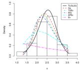
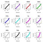
The histogram of the two data sets and the fitted distributions are displayed in Figures S1 and S2, respectively. Further, the P-P plots are displayed in Figures S3 and S4, respectively (see Supplementary Material - appendix A). These plots reveal that the TLOLLEx distribution has a close fit to these data sets.

Table X
Information theoretic criterion for time to failure data.

Distribution	$AIC$	$CAIC$	$BIC$	$HQIC$	$W^{*}$	$A^{*}$
TLOLLEx	163.604	164.271	168.671	165.436	0.0186	0.1382
HEEx	166.754	167.420	171.820	168.586	0.0363	0.2698
MONH	168.691	169.357	173.757	170.522	0.0496	0.3554
BGEx	169.086	170.228	175.841	171.528	0.0465	0.3704
KTEx	172.471	173.614	179.227	174.914	0.0725	0.5422
MOLEx	173.196	173.863	178.263	175.028	0.0853	0.6136
Ga	178.820	179.144	182.198	180.041	0.2052	1.3616
BEx	180.834	181.500	185.900	182.666	0.2054	1.3626
APEx	182.566	182.891	185.944	83.788	0.2187	1.4392
TGEx	183.340	184.007	188.407	185.172	0.2333	1.5194
EEx	184.285	184.609	187.663	185.506	0.2757	1.7600
Ex	228.638	228.743	230.327	229.249	0.2065	1.3689

Table XI
The KS (PV in parentheses) and estimates (SEs in parentheses) for time to failure data.

Distribution	KS	Estimates
TLOLLEx	0.0651	0.0783	13.4838	0.1533
($\lambda ,a,b$ )	(0.9957)	(0.0022)	(0.3049)	(0.0264)
HEEx	0.0936	0.0958	867.518	6.6144
($\alpha ,\vartheta ,\lambda$ )	(0.8739)	(0.1155)	(940.551)	(7.4712)
MONH	0.089	8.6770	0.0280	26.0410
($\alpha ,\lambda ,\vartheta$ )	(0.9040)	(13.8043)	(0.0505)	(16.6133)
BGEx	0.1079	0.1505	235.200	0.2074	32.8356
($a,b,\lambda ,\alpha$ )	(0.7401)	(0.1033)	(290.757)	(0.0880)	(29.7193)
KTEx	0.1059	2.9155	2145.55	0.0334	-0.8222
($a,b,\lambda ,\vartheta$ )	(0.7605)	(1.0753)	(5616.45)	(0.0241)	(0.3080)
MOLEx	0.0910	0.9174	290.353	0.9654
($\alpha ,\vartheta ,\lambda$ )	(0.8944)	(0.9091)	(246.807)	(0.9878)
Ga	0.1277	7.7227	1.2351
($a,b$ )	(0.5311)	(1.6908)	(0.2794)
BEx	0.1283	7.7267	54.6595	0.0213
($a,b,\lambda$ )	(0.5252)	(1.6926)	(56.1355)	(0.0203)
APEx	0.1640	20457.54	0.4460
($\alpha ,\lambda$ )	(0.2318)	(12390.58)	(0.0321)
TGEx	0.1448	8.5465	0.5000	-0.6507
($\alpha ,\lambda ,\vartheta$ )	(0.3707)	(3.1707)	(0.0621)	(0.2560)
EEx	0.1541	9.5142	0.4498
($\alpha ,\lambda$ )	(0.2975)	(2.8959)	(0.0577)
Ex	0.3631	0.1599
($\lambda$ )	(0.000)	(0.0252)

7 - CONCLUSION

In this paper, we have introduced a new three-parameter lifetime model, called Topp-Leone odd log-logistic exponential (TLOLLEx) distribution, which extends the exponential (Ex) distribution. The TLOLLEx PDF can be expressed as a linear mixture of Ex densities. Some of its mathematical properties are discussed. Further, we have discussed different estimation techniques for estimating the unknown parameters of the new distribution. Since it is very difficult to compare these methods theoretically, therefore, we have performed an extensive simulation study in order to identify the best performing estimators. The simulation results show that the ML estimators are the best performing estimators in terms of MSE and MRE for estimating the parameters of the TLOLLEx distribution in comparison with its competitors. The next best performing estimator is the ADE, followed by PCE. Finally, we observe that the TLOLLEx distribution provides better fits than some well-known non-nested models using two real data sets. In conclusion, the TLOLLEx distribution provides a very flexible model for fitting the wide spectrum of positive data sets arising in engineering and lifetime data as well as numerous other fields of scientific investigation.

REFERENCES

• AFIFY AZ, CORDEIRO GM, BUTT NS, ORTEGA EM & SUZUKI AK. 2017. A new lifetime model with variable shapes for the hazard rate. Braz J Proba. Stat 31: 516-541.
• AFIFY AZ, CORDEIRO GM, YOUSOF HM, ALZAATREH A & NOFAL ZM. 2016. The Kumaraswamy transmuted-G family of distributions: properties and applications. J Data Sci 14: 245-270.
• AFIFY AZ, GEMEAY AM & IBRAHIM NA. 2020. The heavy-tailed exponential distribution: risk measures, estimation, and application to actuarial data. Mathematics 8: 1276.
• AFIFY AZ & MOHAMED OA. 2020. A new three-parameter exponential distribution with variable shapes for the hazard rate: estimation and applications. Mathematics 8: 135.
• AFIFY AZ, SUZUKI AK, ZHANG C & NASSAR M. 2019. On three-parameter exponential distribution: properties, Bayesian and non-Bayesian estimation based on complete and censored samples. Commun Stat Simul Comput. (Unpublished) DOI: 10.1080/03610918.2019.1636995.
• AFIFY AZ, ZAYED M & AHSANULLAH M. 2018. The extended exponential distribution and its applications. J Stat Theory Appl 17: 213-229.
• AL-BABTAIN AA, ELBATAL I, AL-MOFLEH H, GEMEAY AM, AFIFY AZ & SARG AM. 2021. The flexible Burr X-G family: properties, inference, and applications in engineering science. Symmetry 13: 474.
• BARRETO-SOUZA W, SANTOS AH & CORDEIRO GM. 2010. The beta generalized exponential distribution. J Stat Comput Simul 80: 159-172.
• BRITO E, CORDEIRO GM, YOUSOF HM, ALIZADEH M & SILVA GO. 2017. The Topp–Leone odd log-logistic family of distributions. J Stat Comput Simul 87: 3040-3058.
• BURNHAM KP & ANDERSON DR. 2002. Model selection and multi-modal inference: a practical information-theoretic approach. Second ed. New York, Springer, 485 p.CHENG R & AMIN N. 1983. Estimating parameters in continuous univariate distributions with a shifted origin. J R Stat Soc Series B Stat Methodol 45: 394-403.
• CORDEIRO GM, AFIFY AZ, ORTEGA EM, SUZUKI AK & MEAD ME. 2019. The odd Lomax generator of distributions: properties, estimation and applications. J Comput Appl Math 347: 222-237.
• DEY S, KUMAR D, RAMOS PL & LOUZADA F. 2017. Exponentiated chen distribution: properties and estimation. Commun Stat Simul Comput 46: 8118-8139.
• GUPTA RD & KUNDU D. 2001. Exponentiated exponential family: an alternative to gamma and Weibull distributions. Biom J: J Math Meth Bio 43: 117-130.
• JONES MC. 2004. Families of distributions arising from distributions of order statistics. Test 13: 1-43.
• KAO JHK. 1958. Computer methods for estimating Weibull parameters in reliability studies. Trans. IRE Reliab Qual Contr 13: 15-22.
• KHAN MS, KING R & HUDSON IL. 2017. Transmuted generalized exponential distribution: a generalization of the exponential distribution with applications to survival data. Commun Stat Simul Comput 46: 4377-4398.
• KUNDU D & RAQAB MZ. 2009. Estimation of R = P(Y < X) for three parameter Weibull distribution. Stat Probab Lett 79: 1839-1846.
• LEMONTE AJ, CORDEIRO GM & MORENO-ARENAS G. 2016. A new useful three-parameter extension of the exponential distribution. Statistics 50: 312-337.
• LOUZADA F, RAMOS PL & PERDONÁ GS. 2016. Different estimation procedures for the parameters of the extended exponential geometric distribution for medical data. Comput Math Methods Med 2016: 1-12.
• MACDONALD P. 1971. An estimation procedure for mixtures of distribution. J R Stat Soc Series B Stat Methodol 33: 326-329.
• MAHDAVI A & KUNDU D. 2017. A new method for generating distributions with an application to exponential distribution. Commun Stat Theory Methods 46: 6543-6557.
• MANSOOR M, TAHIR MH, CORDEIRO GM, PROVOST SB & ALZAATREH A. 2019. The Marshall-Olkin logistic-exponential distribution. Commun. Stat. Theory Methods 48: 220-234.
• NADARAJAH S & KOTZ S. 2006. The beta exponential distribution. Reliab Eng Syst Saf 91: 689-697.
• NASSAR M, AFIFY AZ, DEY S & KUMAR D. 2018. A new extension of weibull distribution: properties and different methods of estimation. J Comput Appl Math 336: 439-457.
• NASSAR M, AFIFY AZ & SHAKHATREH M. 2020. Estimation methods of alpha power exponential distribution with applications to engineering and medical data. Pakistan J Stat Oper Res 16: 149-166.
• PINHO LG.B, CORDEIRO GM & NOBRE JS. 2015. The Harris extended exponential distribution. Commun Stat Theory Methods 44: 3486-3502.
• R CORE TEAM. 2019. R: A Language and Environment for Statistical Computing. R Foundation for Statistical Computing: Vienna, Austria. Available online: https:// www.R-project.org/(accessed on: 26 April 2019).
  » https:// www.R-project.org/
• RASEKHI M, ALIZADEH M, ALTUN E, HAMEDANI GG, AFIFY AZ & AHMAD M. 2017. The modified exponential distribution with applications. Pak J Stat 33: 383-398.
• RODRIGUES GC, LOUZADA F & RAMOS PL. 2018. Poisson–exponential distribution: different methods of estimation. J Appl Stat 45: 128-144.
• SWAIN J, VENKATRAMAN S & WILSON J. 1988. Least squares estimation of distribution function in Johnsons translation system. J Stat Comput Simul 29: 271-297.
• XU K, XIE M, TANG LC & HO SL. 2003. Application of neural networks in forecasting engine systems reliability. Appl Soft Comput 2: 255-268.

Appendix A Figures

Figure S1
Fitted densities for gauge lengths data.

Figure S2
Fitted densities for time to failure data.

Figure S3
The PP plots of the tted models for gauge lengths data.

Figure S4
The PP plots of the tted models for time to failure data.

Publication Dates

• Publication in this collection
  17 Sept 2021
• Date of issue
  2021

History

• Received
  21 May 2019
• Accepted
  11 July 2019